5 Sensing the World: IMUs, Magnetometers, and Barometers
The last two chapters followed energy through the aircraft: out of the pack, through the structure, and into the air. The Anatomy of a Multirotor chapter identified a second chain running alongside it — sensors \(\rightarrow\) flight controller \(\rightarrow\) ESC, closing an attitude loop at several hundred hertz — that carries information rather than power, and that chain begins with a word which has so far gone unexamined. Sensors. Everything the aircraft will ever know about its own orientation, rotation, heading, and height originates in a few grams of micromachined silicon soldered to the flight controller: an inertial measurement unit, a magnetometer, and a barometer. None of these devices measures what the autopilot actually wants. The accelerometer measures the deflection of a microscopic spring; the gyroscope measures energy leaking between two vibration modes; the magnetometer measures a field that the drone’s own power wiring pollutes; the barometer measures a pressure that the propellers themselves disturb. The quantity the control loops need — a smooth, drift-free estimate of the vehicle’s attitude and altitude — exists nowhere on the aircraft as a direct reading. It has to be constructed, at hundreds of times per second, from several noisy, biased, mutually disagreeing measurements.
This chapter follows the data from physics to estimate in three stages. First, what the sensors physically are: how a MEMS accelerometer and gyroscope convert motion into capacitance, why that transduction chain works as well as it does, and where its error sources live. Second, how the measurements get aboard: the two serial buses, I2C and SPI, that carry nearly every sensor stream in embedded robotics, and the bandwidth arithmetic that decides which sensor goes on which bus. Third, how disagreement becomes trust: the complementary filter, derived from the observation that the gyroscope and the accelerometer fail in exactly opposite ways, and the extended Kalman filter that production autopilots run in its place. The treatment is deliberately quantitative, because every rule of thumb in this domain — “gyros drift,” “don’t trust the accelerometer in a turn,” “put the IMU on SPI” — is an arithmetic conclusion wearing a slogan’s clothing.
5.1 Learning Objectives
- Explain what a MEMS accelerometer and a MEMS gyroscope physically measure — proof-mass displacement against a flexure spring, and Coriolis coupling between two vibration modes — and why each output is an inference from Newton’s laws rather than a direct reading of motion.
- Catalogue the principal IMU error sources (bias, bias instability, white noise specified as noise density, temperature drift, and vibration rectification), and compute the attitude error that results from integrating a given gyroscope bias over time.
- Derive the complementary filter from the complementary failure modes of the gyroscope and accelerometer, implement it in a few lines of code, and choose its gain from a desired correction time constant.
- Compare I2C and SPI as sensor buses — wire count, addressing, clock rate, duplex, and DMA compatibility — and use bandwidth arithmetic to justify the topology commonly found on flight controllers: IMU on SPI, magnetometer and barometer on I2C.
- Convert a barometric pressure reading to altitude with the standard-atmosphere formula, estimate the sensor’s resolution in metres, and explain why propeller wash corrupts barometric altitude on a multirotor and what mitigations are used in practice.
5.2 Key Vocabulary
- MEMS (Micro-Electro-Mechanical Systems) — the fabrication technology of etching microscopic mechanical structures — springs, masses, membranes — into silicon alongside the electronics that read them, which is what makes gram-scale, milliwatt-scale inertial sensors possible at consumer prices.
- IMU (Inertial Measurement Unit) — the packaged combination of a three-axis accelerometer and a three-axis gyroscope (sometimes with a magnetometer added, making nine axes), sampled together and timestamped as the primary input to attitude estimation.
- Accelerometer — a sensor that measures specific force: the deflection of a spring-suspended proof mass relative to its housing. At rest it reads 1 g upward (the support force), in free fall it reads zero, and in unaccelerated hover its output vector points away from the Earth — which is precisely what makes it a usable gravity reference.
- Gyroscope — a sensor that measures angular rate. MEMS gyroscopes drive a proof mass into resonant vibration and detect the Coriolis force that rotation couples into an orthogonal sense axis; the output is degrees per second, which must be integrated to yield an angle.
- Magnetometer — a sensor measuring the local magnetic field vector, used to reference the vehicle’s heading (yaw) against the Earth’s field — the one attitude axis that neither the gyroscope nor the accelerometer can stabilize long-term.
- Barometer — a pressure sensor built on a micromachined membrane over a sealed reference cavity, used to infer altitude from the roughly 12 Pa of pressure lost per metre of climb near sea level.
- I2C (Inter-Integrated Circuit, often written I²C) — a two-wire, shared, addressed serial bus: many devices on one data line and one clock line, each selected by a 7-bit address. Wiring-cheap and convenient at modest data rates (100 kbit/s standard, 400 kbit/s fast mode).
- SPI (Serial Peripheral Interface) — a four-wire, full-duplex serial bus with a dedicated chip-select line per device and clock rates commonly in the tens of megahertz, the usual choice where a single sensor must be read fast and often.
- Sensor fusion — the algorithmic combination of multiple imperfect sensors into one estimate better than any of them alone, by exploiting the fact that different sensors fail in different ways at different timescales.
- Complementary filter — the simplest useful fusion algorithm for attitude: a weighted blend \(\hat\theta = \alpha(\hat\theta + \omega\,\Delta t) + (1-\alpha)\,\theta_{\text{accel}}\) that trusts the gyroscope at short timescales and lets the accelerometer’s absolute gravity reference slowly remove the gyroscope’s accumulated drift.
- Noise density — a sensor’s white-noise floor normalized per unit bandwidth (e.g. µg/√Hz or °/s/√Hz); multiplied by the square root of the measurement bandwidth it predicts the RMS noise of the delivered signal, which is why low-pass filtering buys noise reduction at the price of latency.
5.3 What the Flight Controller Must Know
The attitude control loops developed in Part II consume two quantities: the vehicle’s orientation (roll, pitch, yaw) and its angular rates, at update intervals of a few milliseconds. Altitude hold adds a third: height and vertical velocity. The sensor suite maps onto those needs with a deliberate redundancy — every quantity is observable through at least two different physical channels, and no single channel is good enough alone:
- The gyroscope delivers angular rate directly, at kilohertz rates, with low noise — but an angle obtained by integrating rate inherits every error in the rate signal, accumulated without bound.
- The accelerometer delivers the direction of gravity whenever the vehicle is not accelerating — an absolute, drift-free reference for roll and pitch — but it is noisy, and it is corrupted the moment the vehicle maneuvers, because it cannot distinguish gravity from the vehicle’s own acceleration.
- The magnetometer delivers heading against the Earth’s magnetic field — the only absolute reference for yaw, since gravity is silent about rotation around the vertical — but the field it measures is weak (tens of microtesla) and easily polluted by the tens of amperes flowing through the drone’s own power wiring, which is why flight controllers commonly place the magnetometer on the GPS mast, as far from the battery leads as the airframe allows.
- The barometer delivers altitude through pressure — absolute over minutes, but noisy over seconds and disturbed by the propellers’ own airflow.
The pattern to hold onto: each sensor is trustworthy at a timescale where another fails. That asymmetry is not a nuisance; it is the entire basis of sensor fusion, and the rest of the chapter builds toward exploiting it.
5.4 The MEMS Accelerometer: A Spring Scale in Silicon
Mechanically, a MEMS accelerometer is a mass on a spring, etched into a silicon die. A proof mass of tens to hundreds of micrograms is suspended over the substrate by thin silicon flexures — meandering “serpentine” beams anchored to the fixed frame, compliant along the sensing axis and stiff across it. When the package accelerates, the proof mass, by Newton’s first law, initially stays put, so it displaces relative to the housing, stretching one flexure and compressing the other. The system is the classic mass-spring-damper:
\[m\ddot{x} + c\dot{x} + kx = ma,\]
where \(x\) is proof-mass displacement relative to the housing, \(a\) the applied acceleration, \(k\) the flexure stiffness, and \(c\) the damping — largely squeeze-film damping of the gas sealed in the package. Once transients settle, the steady-state displacement is
\[x \approx \frac{m}{k}\,a:\]
the structure converts acceleration into displacement at a fixed, known exchange rate set by geometry. Everything after this is readout. The dominant readout scheme in consumer and robotics-grade parts is capacitive: comb-shaped fingers attached to the proof mass interleave with fixed fingers anchored to the substrate, forming a differential capacitor pair. When the mass deflects, one air gap narrows and the other widens, so \(C_1\) rises as \(C_2\) falls; an on-die ASIC measures \(\Delta C = C_1 - C_2\), which is proportional to \(x\) and therefore to \(a\), then digitizes it and serves it over I2C or SPI. A three-axis part repeats the structure (or arranges electrodes to resolve three axes) on one die.
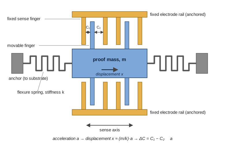
Two consequences of this construction shape everything downstream. First, the accelerometer does not measure coordinate acceleration; it measures specific force — the net non-gravitational force per unit mass acting on the housing. A sensor at rest on a bench reads 1 g pointing up, because the bench pushes up on it; the same sensor in free fall reads zero, because mass and housing fall together and the spring relaxes. This is not a defect. It is exactly what makes the accelerometer a gravity reference: in unaccelerated flight, its output vector points opposite to gravity, and the roll and pitch angles can be recovered from its components by simple trigonometry. The corollary is equally important: during a hard maneuver, the vehicle’s own acceleration adds to that vector, and the “gravity direction” the accelerometer reports is simply wrong. A fusion algorithm must know when not to listen.
Second, the sensing element is a mechanical resonator with microscopic displacements — capacitance changes of femtofarads riding on picofarads. That makes the device sensitive to exactly the environment a multirotor provides: broadband mechanical vibration at the propeller rotation and blade-passing frequencies (about 90 and 181 Hz for the platform sized in the Anatomy chapter). Vibration does not merely add noise; through small nonlinearities in the transduction it can rectify into a false DC offset — an effect examined below — which is why IMU mounting, discussed in the Materials and Power chapter’s stiffness arguments, is a flight-quality issue and not a packaging afterthought.
5.5 The MEMS Gyroscope: Rotation Through the Coriolis Effect
A classical gyroscope stores angular momentum in a spinning rotor; nothing that spins survives miniaturization to silicon, so MEMS gyroscopes use vibration instead. The device — a Coriolis vibratory gyroscope — again suspends a proof mass on flexures, but now drives it electrostatically into sustained resonant oscillation along one axis, the drive mode, like one tine of a tuning fork. When the package rotates at angular rate \(\omega\) about an axis perpendicular to that vibration, each element of the moving mass experiences a Coriolis acceleration
\[\vec{a}_{\text{cor}} = -2\,\vec{\omega} \times \vec{v},\]
where \(\vec{v}\) is the instantaneous drive-mode velocity. That acceleration is perpendicular to both the rotation axis and the drive motion, so it pumps energy into a second, orthogonal sense mode, whose displacement is picked off by capacitive electrodes exactly as in the accelerometer. Because the Coriolis term is linear in \(\omega\), the sense-mode amplitude directly encodes angular rate, and the ASIC delivers a calibrated output in degrees per second.
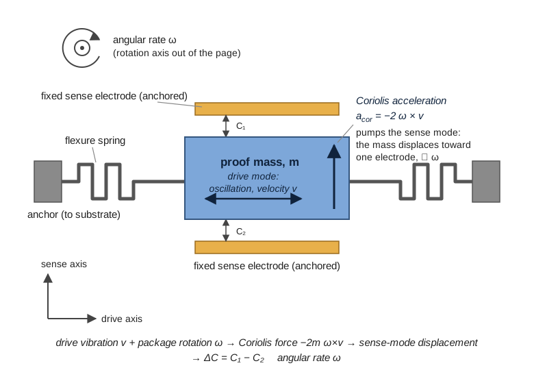
The construction carries its own fine print. The sense signal is proportional to the product of drive velocity and rotation rate, so any wander in drive amplitude appears as a scale-factor error; drive amplitude and flexure stiffness both move with temperature, which is why gyroscope bias and scale factor are specified with temperature coefficients and why the bias you measure at power-on is not the bias you will have ten minutes into a flight, after motor and battery heat have warmed the die. And the structure is, again, a high-Q mechanical resonator living on a vibrating airframe — the same vibration-sensitivity caveat as the accelerometer, sometimes worse, because external vibration near the drive frequency interferes directly with the mechanism.
One more property matters for everything that follows: the gyroscope measures rate, but control and navigation need angle. The only route from one to the other is integration, \(\theta(t) = \theta_0 + \int_0^t \omega\,dt\), and integration is an error amplifier: a constant rate bias \(b\) becomes an angle error \(b\,t\) that grows without limit. The numbers below make that concrete.
5.6 The Barometer: Altitude from a Sealed Cavity
The barometric sensor completes the suite. A micromachined membrane is suspended over a cavity sealed at a reference pressure; ambient pressure flexes the membrane, and the deflection is read capacitively or piezoresistively, temperature-compensated on-chip against factory calibration coefficients, and served over the same buses. Devices of the widely used Bosch BMP280/BMP388 class resolve pressure to roughly ±0.12 hPa relative — and the reason that number is interesting is what it converts to in metres.
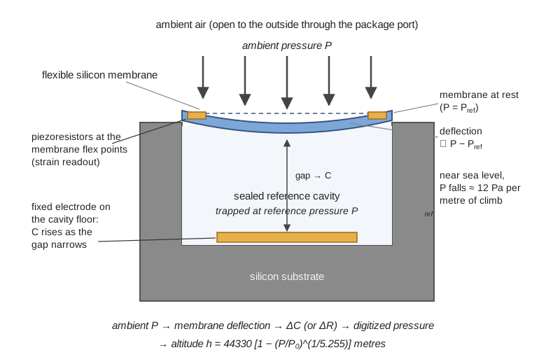
Hydrostatic equilibrium sets the exchange rate. Pressure falls with height as \(dP/dh = -\rho g\); with sea-level air density \(\rho \approx 1.225\ \text{kg/m}^3\), that is \(1.225 \times 9.81 \approx 12\ \text{Pa}\) per metre. A ±0.12 hPa (±12 Pa) sensor therefore resolves altitude to about ±1 m — good enough for altitude hold, nowhere near good enough for landing flare or obstacle clearance. Over larger height changes, density itself falls with altitude, and integrating the hydrostatic relation through the standard-atmosphere temperature lapse yields the practical closed form used in flight-controller code:
\[h = 44330\left[1 - \left(\frac{P}{P_0}\right)^{1/5.255}\right]\ \text{metres},\]
with \(P_0\) the reference pressure. Worked through: if the reference is 101,325 Pa and the sensor now reads 100,725 Pa, then \(P/P_0 = 0.99408\), the bracket evaluates to \(1 - 0.99408^{0.1903} = 0.001129\), and \(h = 44330 \times 0.001129 \approx 50.1\ \text{m}\) — matching the linear 600 Pa ÷ 12 Pa/m estimate, as it should for a small height change.
The formula’s fine print is operationally important. \(P_0\) is not a constant of nature; local sea-level-equivalent pressure moves with the weather by amounts that dwarf the sensor’s resolution (a modest pressure system shift of 3 hPa masquerades as 25 m of altitude). Flight controllers therefore use the barometer relatively: record the pad pressure at arming as \(P_0\), and report height above the launch point, fusing GPS altitude in the background to restrain slow drift. And on a multirotor the sensor has a further, self-inflicted problem: it sits inside the turbulent flow field of its own propellers. Prop wash, ground effect near the pad, and throttle transients all modulate the local static pressure, appearing as spurious altitude excursions precisely during takeoff and landing. The standard mitigations are physical and computational together: flight controllers typically shroud the barometer under open-cell foam, which damps turbulent pressure fluctuations while passing the slow static signal, and apply low-pass filtering plus estimator-level fusion so that short-term barometric excursions are outvoted by the inertial sensors’ vertical-acceleration evidence.
5.7 Why the Raw Data Cannot Be Trusted
Every error a fusion algorithm must fight can be read off an IMU datasheet, and it is worth doing so once with real numbers. The Bosch BMI088 — an IMU designed for drones and marketed for exactly the vibration environment described above — specifies, in round figures: accelerometer zero offset ±20 mg typical; gyroscope zero offset ±1 °/s typical, with temperature coefficient ±0.015 °/s per kelvin; gyroscope noise density 0.014 °/s/√Hz; accelerometer noise density 175 µg/√Hz. Four distinct failure modes hide in those lines.
Bias. The output at zero true input is not zero. A ±1 °/s gyro bias, integrated naively, is an attitude error growing at 60 degrees per minute — a horizon that rolls over in ninety seconds while the aircraft sits still on the bench. Autopilots therefore calibrate the bias at every boot by averaging the output while the vehicle is stationary. But calibration only removes the bias as it was at boot: with a temperature coefficient of ±0.015 °/s/K, a die that warms 20 K during flight — routine, with motors and battery working — can acquire up to 0.3 °/s of fresh bias, worth 18 degrees of accumulated error per minute of pure integration. Bias is not a constant to be subtracted once; it is a slowly moving target, which is exactly why production estimators track it as a state (below) rather than a calibration value.
White noise. Thermomechanical and electronic noise set a floor that no calibration touches; it can only be traded against bandwidth. Noise density makes the trade quantitative: RMS noise equals density times the square root of bandwidth. Sampled with a 100 Hz bandwidth, the BMI088’s gyro shows \(0.014 \times \sqrt{100} = 0.14\) °/s RMS — negligible for rate control. The accelerometer shows \(175\ \text{µg} \times \sqrt{100} = 1.75\) mg RMS, which corrupts a gravity-derived tilt angle by roughly \(\arcsin(0.00175) \approx 0.1°\) — small, but only because the bandwidth was kept narrow. Widen the filter to catch faster dynamics and the noise grows as \(\sqrt{\text{bandwidth}}\); the accelerometer’s tilt estimate is inherently a slow reference.
Vibration rectification. A perfectly symmetric sinusoidal vibration should average to zero. Through the sensor’s small nonlinearities it does not: sustained vibration produces a net DC shift in the output — vibration rectification error, specified in datasheets as bias per g² of vibration. On a multirotor feeding the IMU continuous excitation at 90 and 181 Hz, this converts propeller imbalance directly into attitude bias. The defenses are layered: balance the propellers (reduce the source), soft-mount the flight controller or IMU (attenuate the path — the mechanical low-pass filter of the Anatomy chapter), keep frame resonances away from the excitation bands (the Materials chapter’s stiffness argument), and apply software notch filters keyed to measured motor RPM (remove what remains). Only after all four does the noise floor approach what the datasheet promised.
Scale factor and cross-axis error. The gain from true input to output deviates slightly from nominal and drifts with temperature, and a rotation about one axis leaks fractionally into the others through imperfect axis alignment. Both are percent-level effects, calibrated at the factory and refined by the estimator; they matter mostly for aggressive maneuvers, where a 1 % scale error on a 360°/s roll is 3.6°/s of phantom rate.
5.8 Getting the Data Aboard: I2C versus SPI
Between the sensor die and the autopilot’s memory sits a serial bus, and the choice of bus is a genuine engineering decision, not a wiring detail. The two candidates on virtually every flight controller:
| Property | I2C | SPI |
|---|---|---|
| Wires | 2 shared (SDA data, SCL clock), open-drain with pull-up resistors | 4 (clock, master-out, master-in) plus one dedicated chip-select line per device |
| Device selection | 7-bit address in-band; many devices share the same two wires | Chip-select wire per device; pin count grows with device count |
| Clock rate | 100 kbit/s standard, 400 kbit/s fast mode, 1 Mbit/s fast-mode-plus | Commonly single-digit to tens of MHz; modern IMUs typically accept 10–24 MHz |
| Duplex | Half — the wire turns around between write and read | Full — data flows both directions simultaneously |
| Scaling limit | Bus capacitance and pull-up sizing degrade edges as devices and trace length grow | Wiring only; each device’s bandwidth is independent, no arbitration |
| DMA streaming | Workable but awkward at high rates | Natural fit — burst reads at kilohertz rates without CPU involvement |
The arithmetic that settles the question for the IMU: a six-axis sample is 12 data bytes (three 16-bit words each for accelerometer and gyroscope). Reading it over I2C costs, with addressing, register pointer, ACK bits, and start/stop overhead, roughly 130 bit-times per transaction — about 325 µs at 400 kbit/s. That caps a lone IMU at roughly 3 kHz while consuming the entire shared bus, and modern rate controllers want gyro samples at 1–8 kHz with time left over for every other device on the wire. The same 12-byte burst over SPI at 10 MHz completes in about 10 µs, more than thirtyfold faster, full-duplex, and DMA-driven so the CPU never touches the transfer. This is why flight controllers of the Pixhawk and Betaflight class typically wire the primary IMU to a dedicated SPI bus.
The magnetometer and barometer invert every term of that argument. Heading and altitude change slowly; both sensors are commonly read at 10–100 Hz, three orders of magnitude below the gyro. At those rates I2C’s bandwidth is ample, and its strengths dominate: two wires shared among several devices, in-band addressing so a compass, a barometer, and a battery monitor coexist without extra pins, and easy extension over the longer run to a mast-mounted GPS/compass module. Hence the hybrid topology found on most flight controllers: fast, lonely sensor on SPI; slow, sociable sensors on I2C. The general lesson generalizes well beyond drones — bus selection is the required sample rate, the device count, and the pin budget, evaluated in that order.
5.9 Sensor Fusion: The Complementary Filter
Now the punchline the chapter has been assembling. The gyroscope integrates into a smooth, responsive angle that drifts without bound; the accelerometer supplies an absolute, drift-free angle that is noisy and lies during maneuvers. One fails slowly, the other fails fast — so blend them, each at the timescale where it is trustworthy. For one axis (pitch, say), with gyro rate \(\omega\), sample interval \(\Delta t\), and \(\theta_{\text{accel}}\) the tilt angle computed from the accelerometer’s gravity vector by trigonometry:
\[\hat{\theta}_{k} = \alpha\left(\hat{\theta}_{k-1} + \omega_k\,\Delta t\right) + (1 - \alpha)\,\theta_{\text{accel},k},\]
with gain \(\alpha \in [0,1]\) chosen close to 1. Each step trusts the gyro’s propagation almost entirely — preserving its smoothness and responsiveness — while the small \((1-\alpha)\) correction leaks the accelerometer’s absolute reference in, continuously bleeding off whatever drift the integration has accumulated. In the frequency domain the structure explains the name: the gyro path is high-pass filtered, the accelerometer path low-pass filtered, and the two responses are complementary — they sum to unity, so no frequency band is lost, merely assigned to the sensor that handles it best.
The gain is not arbitrary; it encodes a time constant. The accelerometer correction acts as a first-order pull toward \(\theta_{\text{accel}}\) with
\[\tau = \frac{\alpha\,\Delta t}{1-\alpha}.\]
Run the filter at 250 Hz (\(\Delta t = 4\) ms) with \(\alpha = 0.99\) and \(\tau \approx 0.4\) s: gyro drift is corrected on a timescale of half a second, while accelerometer noise and maneuver corruption faster than that are averaged away. Choosing \(\alpha\) is choosing where to place the crossover between the two sensors’ credibility — lower \(\alpha\) tracks the gravity reference more tightly but lets accelerometer noise and the vehicle’s own accelerations bleed into the attitude; higher \(\alpha\) rides the gyro longer but corrects drift more slowly. Typical values sit between 0.90 and 0.99 depending on sample rate and vibration environment.
The algorithm is short enough to be shown whole:
import math

class ComplementaryFilter:
    """Single-axis pitch estimator fusing gyro rate with accel tilt."""

    def __init__(self, alpha: float = 0.99):
        self.alpha = alpha
        self.pitch = 0.0          # radians

    def update(self, gyro_rate: float, ax: float, az: float,
               dt: float) -> float:
        # 1. Propagate with the gyro (trusted short-term).
        pitch_gyro = self.pitch + gyro_rate * dt
        # 2. Absolute tilt from the gravity vector (trusted long-term).
        pitch_accel = math.atan2(ax, az)
        # 3. Blend: high-pass the gyro path, low-pass the accel path.
        self.pitch = (self.alpha * pitch_gyro
                      + (1.0 - self.alpha) * pitch_accel)
        return self.pitch
Yaw needs one more ingredient: gravity says nothing about rotation around the vertical, so the absolute reference for the third axis comes from the magnetometer — the same blend, with a tilt-compensated compass heading standing in for \(\theta_{\text{accel}}\). And one caveat must be carried forward: \(\theta_{\text{accel}}\) is only the true tilt when the vehicle is unaccelerated. During a sustained coordinated maneuver the accelerometer’s vector tilts with the maneuver, and the filter slowly follows it into error. Keeping \(\alpha\) high limits the damage; fixing it properly requires knowing how much to trust each measurement moment by moment — which is precisely the upgrade the Kalman filter provides.
5.9.1 From Blend to Estimator: The EKF
Production autopilots do not fly on complementary filters. PX4’s default estimator, EKF2, is an extended Kalman filter that carries roughly two dozen states — attitude as a quaternion, three-axis velocity and position, and the gyroscope and accelerometer biases themselves, along with magnetic field and wind states — and fuses IMU, magnetometer, barometer, GPS, and optionally rangefinder and optical flow, each stream weighted by a continuously updated estimate of its own uncertainty. The conceptual advances over the fixed-\(\alpha\) blend are three. The filter estimates the biases rather than averaging them out, so the slow bias wander that defeats boot-time calibration is tracked and removed in flight. It replaces the fixed gain with a covariance: each sensor’s influence at each instant is proportional to how trustworthy the filter currently computes it to be, so a GPS glitch or a maneuver-corrupted accelerometer sample is automatically down-weighted. And it monitors innovations — the gap between what a sensor reports and what the filter predicted it would report — which turns the estimator into a fault detector: a failing magnetometer announces itself statistically before it can steer the vehicle wrong. The complementary filter remains the right first implementation — transparent, tunable, sufficient for a bench demonstrator — and the right mental model for what the EKF is doing beneath its matrices.
This estimate is also where the chapter’s material surfaces in the running example. The Systems Architecture chapter in Part V picks up the pipeline from the consumer’s side: the Goose Management System’s Failsafe node — the independent monitor that watches battery state and separation distance and can override whatever is flying the aircraft — does not read raw sensors at all, but consumes the fused attitude and position estimates published by the flight controller’s onboard EKF, trusting the estimator to have already fought every battle described here. When that chapter asks what happens if the estimate itself degrades, the error budget assembled above is the vocabulary the answer is written in.
5.10 Check Your Understanding
- An accelerometer sitting motionless on a bench reads 1 g pointing up; the same accelerometer in free fall reads zero. Explain both readings from the proof-mass mechanism, and state precisely what physical quantity the sensor measures.
The sensor measures the displacement of a spring-suspended proof mass relative to its housing, which responds to specific force — the net non-gravitational force per unit mass on the housing. On the bench, the bench pushes the housing up with 1 g of support force while gravity acts equally on housing and proof mass; the spring must supply the proof mass’s share, deflecting by \((m/k)g\) — hence a 1 g reading pointing up. In free fall, gravity accelerates housing and proof mass identically, no spring force is needed, the mass rides centered, and the output is zero. The practical consequence: in unaccelerated flight the output vector points opposite gravity, making the accelerometer an absolute tilt reference — but only when no other acceleration is present.
- A gyroscope is bias-calibrated at boot, but during flight the die warms 15 K. Using the BMI088’s temperature coefficient of ±0.015 °/s/K, bound the fresh bias and the resulting attitude error after 4 minutes of pure gyro integration. What does this imply about bias as a “calibrate once” quantity?
Fresh bias: up to \(15 \times 0.015 = 0.225\) °/s. Integrated for 4 minutes: \(0.225 \times 240 = 54°\) of attitude error — a horizon rolled halfway to vertical, from temperature drift alone, on a sensor that was perfectly calibrated at boot. Bias is therefore a slowly moving target, not a constant: boot-time calibration removes only its value at boot. This is why a drift-correcting fusion mechanism must run continuously (complementary filter at minimum), and why production estimators like PX4’s EKF2 go further and carry the gyro biases as estimated states, tracking their wander throughout the flight.
- A complementary filter runs at 500 Hz and should correct gyro drift with a time constant of about 0.5 s. Compute the required gain \(\alpha\), and describe qualitatively what changes if \(\alpha\) is lowered to 0.95.
From \(\tau = \alpha\,\Delta t/(1-\alpha)\) rearranged, \(\alpha = \tau/(\tau + \Delta t) = 0.5/(0.5 + 0.002) \approx 0.996\). Lowering \(\alpha\) to 0.95 at \(\Delta t = 2\) ms gives \(\tau = 0.95 \times 0.002/0.05 = 38\) ms: the filter now yanks the estimate toward the accelerometer within a few tens of milliseconds. Drift correction is far more aggressive, but accelerometer white noise passes almost unfiltered into the attitude, and every maneuver’s linear acceleration — which tilts the measured “gravity” vector — corrupts the estimate almost immediately. The gain sets the crossover frequency between the two sensors’ credibility, and 38 ms is far below the timescale on which the accelerometer can be trusted.
- A six-axis IMU sample is 12 data bytes, and the rate controller wants it at 2 kHz. A colleague proposes putting the IMU on the flight controller’s I2C bus (400 kbit/s fast mode) alongside the barometer and compass. Evaluate the proposal with arithmetic, and state the topology actually used.
With addressing, register pointer, ACKs, and start/stop framing, each 12-byte read costs roughly 130 bit-times — about 325 µs at 400 kbit/s. At 2 kHz the IMU alone demands \(2000 \times 325\ \text{µs} = 0.65\) s of bus time per second — 65 % of the shared bus, before the barometer or compass sends a byte; at higher gyro rates the demand exceeds the bus outright. The proposal fails. The standard topology puts the IMU alone on SPI — where a 10 MHz clock moves the burst in about 10 µs, full-duplex and DMA-driven — and leaves the slow, low-rate barometer and magnetometer sharing I2C, where two-wire wiring and in-band addressing are worth more than bandwidth.
- At arming, the barometer reads 101,325 Pa, recorded as \(P_0\). Later it reads 100,725 Pa. Compute the altitude gain both by the linear approximation and by the standard-atmosphere formula, and explain why the flight controller uses launch-point-relative rather than absolute barometric altitude.
Linear: \(\Delta P = 600\) Pa at \(\approx 12\) Pa/m gives \(\approx 50\) m. Exact: \(h = 44330[1-(100725/101325)^{1/5.255}] = 44330 \times 0.001129 \approx 50.1\) m — the two agree, as they must for small height changes. Absolute altitude is avoided because the formula’s reference pressure is weather-dependent: local sea-level-equivalent pressure routinely shifts by several hPa as systems move through, and a 3 hPa shift masquerades as roughly 25 m of altitude. Recording the pad pressure at arming cancels the weather term at the moment of takeoff, leaving only its slow drift during the flight — which the estimator restrains by fusing GPS altitude.
- During takeoff, a quadcopter’s barometric altitude briefly reads below the pad it just left. Give the physical cause, and name one physical and one computational mitigation.
The barometer measures local static pressure, and near the ground the propellers’ wash — intensified by ground effect — swirls turbulent, dynamically disturbed air over the sensor’s port. A transient pressure rise at the port reads as a drop in altitude, regardless of what the vehicle is doing. Physical mitigation: shroud the sensor under open-cell foam (and mount it away from direct prop wash), damping fast turbulent fluctuations while passing the slow static-pressure signal. Computational mitigation: low-pass filter the pressure stream and, more fundamentally, fuse barometric altitude with inertial vertical acceleration (and GPS) in the estimator, so a pressure excursion unsupported by accelerometer evidence is discounted rather than believed.
5.11 Try It
Part 1 — meet your sensor’s noise. Take any IMU you can log — a flight controller, a phone, or a breakout board — and capture a minute of raw accelerometer and gyroscope data with the device perfectly still. Compute each channel’s mean (the bias) and standard deviation (the RMS noise), and compare the noise against the datasheet’s noise density times the square root of your effective bandwidth; they should agree within a factor of two, and understanding why yours differs is half the exercise. Then integrate the raw gyro rate numerically and plot the resulting “attitude” of the motionless sensor over five minutes: the drift you watch accumulate is the failure mode this whole chapter exists to fix. Finally, subtract the measured bias and integrate again — and note that the drift is reduced but not gone, which is the temperature-wander argument made empirically.
Part 2 — build the filter and try to break it. Implement the complementary filter above against your logged (or live) data stream and plot three traces together: integrated gyro alone, accelerometer tilt alone, and the fused estimate. Tilt the board smoothly, hold it still, then shake it. Identify each raw estimator’s characteristic failure in the traces — drift in one, noise and shake-corruption in the other — and verify the fused trace inherits neither. Then sweep \(\alpha\) through 0.80, 0.95, and 0.99, computing the implied time constant for each, and write two or three sentences stating which value you would fly and why. If you have access to a flight controller, finish with a bus audit: from its documentation or schematic, list which bus each sensor sits on, and justify the designer’s choices with the bandwidth arithmetic from this chapter.
Related Lab: See Appendix B for the lab assignment that applies this chapter’s concepts.