14 TinyML: Deploying Neural Networks on Embedded Hardware
The Images as Data chapter closed on a promise with two halves: how a network’s kernel weights are learned, and how a network of them is compressed until it runs, at frame rate, inside a 10-watt computer bolted to a 2.2-kilogram aircraft. This chapter takes the second half first, and the order is deliberate. Learning the weights — the data, the labels, the training loop — is the business of the next chapter, on building a detection pipeline; but what can usefully be trained is dictated by where the result must run, and an engineer who trains first and asks deployment questions afterward routinely produces a model that is accurate, elegant, and unflyable. The discipline that takes the deployment constraints as the starting point of model design has a name: TinyML — machine learning made useful under physical constraints of memory, compute, power, and time. Its founding observation is a mismatch. Mainstream deep learning grows by every axis at once — more parameters, more data, more accelerator hours — while an aircraft’s budget is fixed by battery chemistry and payload mass before any model is chosen. Someone must move, and it will not be the battery.
The constraints themselves are not new to this book. Part I priced the wireless link and found it could not carry the camera stream, which is why the pixels are understood onboard at all; the Anatomy of a Multirotor chapter allotted roughly 12 W to the entire avionics complement and showed that every added gram reappears as lost loiter time; and the previous chapter left a warning on the table: the tensors flowing between a network’s layers often cost more memory than the network’s own weights. What this chapter adds is the machinery that lives inside those constraints. It maps the three places a model can run and why the choice among them precedes every other choice; it itemizes the real memory bill of onboard inference — weights, activations, buffers — rather than the datasheet’s flattering summary; it develops quantization, the single most consequential compression technique, from its arithmetic up through a worked accounting of what it saves; it surveys pruning and distillation, the other members of the compression toolbox; and it follows a trained model down the deployment pipeline — convert, optimize, deploy — through the runtimes that execute it, ending with a comparison of the two toolkits that dominate the smallest tier of that pipeline, TensorFlow Lite for Microcontrollers and Edge Impulse.
14.1 Learning Objectives
- Place a given computation on the right tier of the drone compute hierarchy — cloud, companion computer, or microcontroller — by arguing from latency, bandwidth, power, link reliability, and privacy, and explain why training and inference almost never share a tier.
- Itemize the memory bill of onboard inference as weights, activations, and buffers, estimate each from a model’s architecture and input shape, and identify which term dominates on each hardware tier.
- Explain what int8 quantization does mechanically — the scale factor, the rounding, the 256 levels — and compute the memory saving for a specific layer and a whole model at float32 versus int8.
- State why quantization typically improves latency and energy per inference, not just footprint, and what accuracy cost it exacts and how calibration and quantization-aware training contain that cost.
- Describe pruning and knowledge distillation, and state the runtime-support caveat that separates a smaller model file from a faster model.
- Compare Edge Impulse and TensorFlow Lite for Microcontrollers as deployment toolkits — who owns each pipeline stage, what each is optimized for, and which engineering situations favor each.
14.2 Key Vocabulary
- TinyML — the discipline of designing, compressing, and deploying machine-learning models to run under tight physical constraints — memory in kilobytes to megabytes, power in milliwatts to watts — on hardware at or near the sensor that produces the data.
- Quantization — replacing a model’s high-precision numbers (typically 32-bit floats) with low-precision ones (typically 8-bit integers) related by a stored scale factor, cutting memory, memory bandwidth, and usually latency at a small cost in accuracy.
- Post-training quantization (PTQ) — quantizing an already-trained float model by measuring the ranges of its weights and activations on a small calibration dataset and choosing scale factors from them; no retraining required.
- Quantization-aware training (QAT) — training (or fine-tuning) a model with simulated quantization in the loop, so the weights settle into values that survive rounding; costlier than PTQ but recovers most of its accuracy loss.
- Pruning — removing weights, channels, or whole neurons that contribute little to a network’s output; shrinks the parameter count, but yields speed only when the runtime and hardware can exploit the resulting sparsity or reduced structure.
- Knowledge distillation — training a small student model to reproduce the outputs of a large teacher model, transferring capability into a deployable size; the teacher stays on the workstation, the student flies.
- Model footprint — the storage a deployed model occupies (its weights plus metadata), as distinct from the RAM its execution consumes; the number quoted on a model card, and never the whole bill.
- Activation memory — the RAM occupied at inference time by the intermediate tensors flowing between layers; it scales with input resolution and often exceeds the weights, especially on memory-poor devices.
- Inference latency — the wall-clock time from presenting an input tensor to receiving the model’s output, the quantity a control loop actually waits on; measured, never assumed, and the central subject of the Real-Time Inference on the Edge chapter.
- TensorFlow Lite (TFLite) — the deployment-oriented branch of the TensorFlow ecosystem: a converter that emits a compact model file and a lean runtime that executes it on phones and single-board computers; its sibling TensorFlow Lite for Microcontrollers (TFLM) is a C++ library that runs the same models on bare-metal microcontrollers with no operating system and no dynamic memory allocation.
- Edge Impulse — a hosted end-to-end platform for embedded ML that carries a project from data acquisition through signal processing, training, and testing to an exported, compiled C++ library for a target microcontroller.
- Tensor arena — in TFLM, the single statically allocated block of RAM from which all of a model’s activations and scratch buffers are carved at runtime; the developer sizes it by hand, and it is the practical measure of a model’s RAM appetite on an MCU.
14.3 The Placement Problem
Every machine-learning system that touches a robot answers one question before any question of architecture: where does the model run? The candidate answers form a hierarchy of three tiers, separated by orders of magnitude in every resource that matters, and Figure 14.1 lays them side by side.
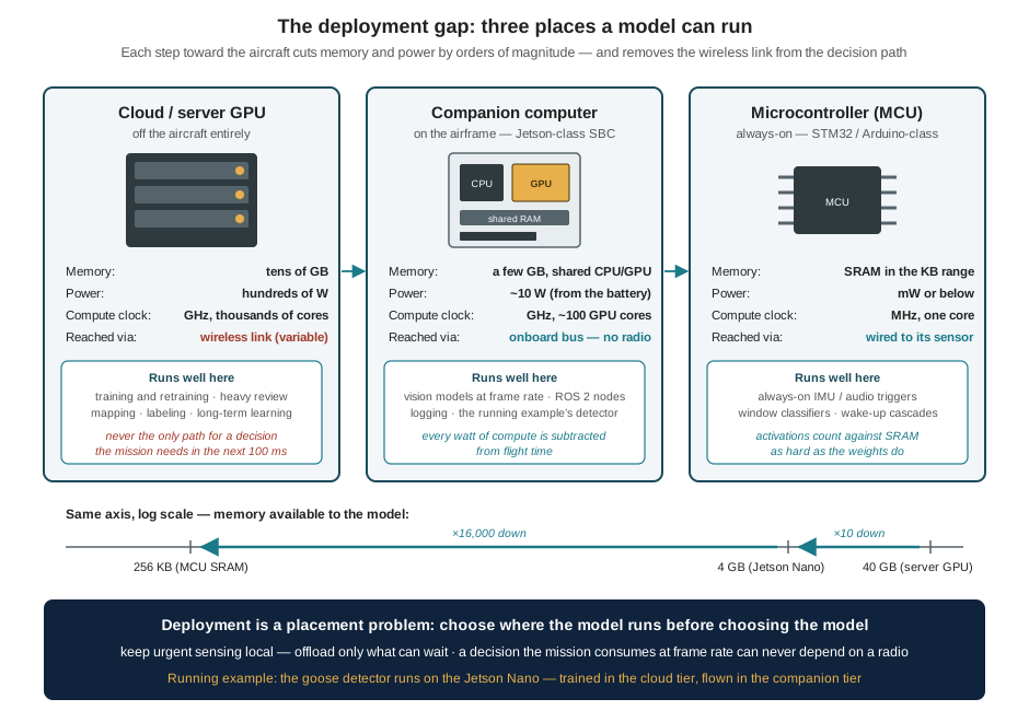
At the top sits the cloud tier — server GPUs with tens of gigabytes of memory, drawing hundreds of watts, reachable from the aircraft only through a wireless link. Part I already disqualified that link as a pipe for imagery on bandwidth grounds; the placement argument adds two counts to the indictment. The first is latency and its variance: a round trip over a real wireless link takes tens to hundreds of milliseconds when it works, and an unbounded time when it degrades — and a deterrence maneuver steering toward a moving animal consumes a fresh target position every frame. A decision loop is only as fast as its slowest hop, and a hop through a radio makes the loop’s worst case the radio’s worst case. The second is power: transmitting data costs battery just as computing does, and streaming sensor data to remote compute spends the energy budget twice — once to send the question, once to fly while waiting for the answer. The cloud tier is not thereby useless; it is where everything that can wait belongs — training and retraining, heavy post-flight analysis, mapping, labeling, the long-term learning loop. The design rule the hierarchy enforces is exactly that split: keep urgent sensing local; offload only what can wait.
The middle tier is the companion computer, and it is where this book has been heading since Part I bolted one to the airframe. A Jetson-class single-board computer offers a few gigabytes of RAM shared between CPU and GPU, roughly a hundred GPU cores, and a power appetite near 10 W — a budget the Companion Computers chapter showed already strains the ~12 W avionics allowance. It runs a full Linux stack, ROS 2 nodes, and — decisively — GPU-shaped inference at frame rate, with no radio between the camera and the decision. This is the tier the running example’s detector occupies, and the tier whose constraints shape most of this chapter.
The bottom tier is the microcontroller (MCU) — an STM32- or Arduino-class chip clocked in megahertz, holding SRAM measured in kilobytes, drawing milliwatts. No deep vision model fits here, and none should be forced to; the tier’s genius is different. An MCU can afford to be always on: a 1-D convolutional classifier watching an accelerometer window for anomalous vibration, or an audio trigger listening for a signature, can run continuously for the cost of a status LED and wake heavier machinery only when something warrants it. The source constraint that defines this tier is worth internalizing as a single figure of merit: a MobileNet-class vision model occupies about 16.9 MB as trained, while a realistic MCU memory budget is 256 KB — a factor of sixty-six before a single activation or buffer is counted. Deployment at this tier is not a matter of trimming a model; it is a matter of designing a different, far smaller one, which is why the toolkits examined at this chapter’s end exist.
Two consequences of the hierarchy organize everything that follows. First, training and inference split across tiers. Training a network — thousands of gradient-descent passes over a dataset — is exactly the bursty, deadline-free, compute-hungry workload the cloud tier exists for, and it happens once; inference happens on every frame, forever, under a deadline, and must live onboard. The pipeline connecting the two tiers — train on a workstation, convert, optimize, deploy, infer — is this chapter’s final subject. Second, placement precedes architecture. The question “what is the smallest model and sensor configuration that is useful enough for the mission?” has a different answer on each tier, so an engineer who has not chosen the tier cannot meaningfully choose the model. The tier fixes the budget; the budget is mostly memory and time; and the memory budget deserves to be itemized before anything is compressed to fit it.
14.4 The Memory Bill: Weights, Activations, Buffers
Ask what a model costs to run and the usual answer is its parameter count — “a 3.2-million-parameter detector” — converted at four bytes per float32 weight to a model footprint of 12.8 MB. That number is real, but treating it as the memory requirement is the embedded-ML equivalent of budgeting a vehicle by its sticker price. What the device must actually hold at the moment of inference is closer to
\[ \text{RAM peak} \approx \text{activations} + \text{input buffers} + \text{runtime workspace} + \text{application state}, \]
with the weights alongside — and on most platforms the largest term is not the weights. It is the activations: the intermediate tensors flowing between layers, which the Images as Data chapter flagged as the hidden cost of input resolution and which can now be made precise. Consider the first convolutional layer of a detector taking a 640 × 640 × 3 input: a bank of 32 kernels at stride 2 produces a 320 × 320 × 32 feature map. The layer’s weights are trivial — \(3 \times 3 \times 3 \times 32 = 864\) of them, under 4 KB as float32. Its output is not:
\[ \begin{aligned} 320 \times 320 \times 32 &= 3{,}276{,}800\ \text{values} \\ \text{as float32:}\quad 3{,}276{,}800 \times 4\ \text{B} &\approx 13.1\ \text{MB}. \end{aligned} \]
One layer, near the top of the network, transiently holds more than three thousand times its own weight in activations — and at least two such tensors are alive at any moment, since a layer’s input must persist while its output is written. Activation memory decays as the network’s spatial dimensions shrink deeper in, so the peak usually sits in these wide early layers, and the peak is what must fit. To the weights and activations add the buffers an application owns because it is a robot and not a benchmark: the camera frames themselves (at the 640 × 480 mode of the Images as Data chapter, 921,600 bytes each, and a capture pipeline holds more than one), the runtime’s scratch workspace, and the state of the application around the model. Figure 14.2 draws the full bill for an illustrative small detector, and its shape explains most of embedded-ML practice.
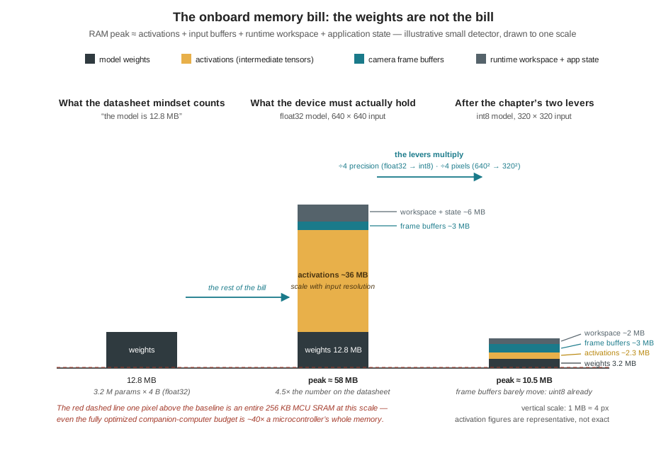
Three lessons fall out of the figure. First, the two big levers multiply: quantizing values from float32 to int8 divides both weights and activations by four, and halving the model’s input side divides activations (and compute) by four again — together taking the illustrative peak from ~58 MB to ~10 MB. The resolution lever is the same one the Images as Data chapter priced from the other side: every halving also halves the pixels on a distant goose, so the lever is pulled against the mission’s detection range, not freely. Second, some terms do not move: camera frames arrive as uint8 and cannot be quantized further, so a bill dominated by buffers responds to pipeline design (fewer copies, smaller queues, streaming windows instead of stored histories) rather than model compression. Third, the tiers reprice the bill. On a 4 GB Jetson sharing memory between CPU, GPU, and the whole operating system, a 58 MB peak is affordable and the bill’s real bite is bandwidth — every byte of weights and activations must move through memory for every frame, and moving bytes costs time and energy. On a 256 KB MCU the same accounting is existential: the entire stacked bar must fit in SRAM, which is why the canonical MCU vision demonstration is a 96 × 96 grayscale classifier occupying a few hundred kilobytes, and why the slide from megabytes to kilobytes cannot be walked by compression alone. It begins, on every tier, with the same first step: giving up 24 of the 32 bits every number is carrying.
14.5 Quantization: Trading Precision for Feasibility
A trained network’s weights are float32 values: 32 bits encoding a sign, an exponent, and 23 bits of mantissa, able to distinguish on the order of \(10^{38}\) magnitudes with seven decimal digits of precision. Training genuinely uses that dynamic range — gradient updates are tiny nudges accumulated over thousands of steps, and they vanish if the representation cannot resolve them. Inference does not. A finished network is a fixed function being evaluated, not adjusted; its decisions rest on comparisons — which class score is largest, whether a confidence clears a threshold — and comparisons survive small perturbations of every number involved. Empirically, the weights of a trained layer huddle in a narrow, roughly bell-shaped band (a range like \([-0.4, +0.4]\) is typical), occupying a sliver of float32’s range. Thirty-two bits are being spent to store values that a much coarser code could carry. Quantization is that coarser code.
The standard scheme maps each float value \(r\) to an 8-bit integer \(q\) through an affine relation:
\[ r \approx S \,(q - Z), \]
where the scale \(S\) is a float32 constant and the zero point \(Z\) is the integer to which the real value 0.0 maps. For weights, which are centered near zero, the symmetric special case \(Z = 0\) suffices, and the scheme collapses to \(r \approx S q\): choose \(S\) so that the largest-magnitude weight lands on the integer extreme, and every weight becomes \(q = \operatorname{round}(r/S)\), an integer in \([-128, 127]\). Figure 14.3 traces the mapping for a concrete layer — the measured weight range sets \(S\), one worked weight is quantized and dequantized, and the rounding error is bounded — and then presents the bill.
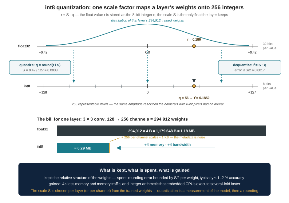
The accounting deserves to be walked once by hand, because it is the worked answer to a question the compression literature usually leaves qualitative. Take a mid-network detection layer: a 3 × 3 convolution from 128 input channels to 256 output channels. Its weight count and float32 cost are
\[ \begin{aligned} 3 \times 3 \times 128 \times 256 &= 294{,}912\ \text{weights} \\ \text{as float32:}\quad 294{,}912 \times 4\ \text{B} &= 1{,}179{,}648\ \text{B} \approx 1.18\ \text{MB}. \end{aligned} \]
Quantized, each weight is one byte — 294,912 bytes, about 0.29 MB — plus the metadata that makes the integers meaningful: one scale per output channel (per-channel scaling tracks the fact that different kernels settle into different ranges), \(256 \times 4\ \text{B} \approx 1\) KB. The overhead is a rounding error on the total; the saving is a clean factor of four, and it compounds across the model: the 16.9 MB MobileNet of the previous section is about 4.2 million float32 weights at four bytes each, and the same network quantized is about 4.2 MB. What was spent to earn it is bounded and small: each weight moved by at most \(S/2 \approx 0.0017\) — noise at the scale of the weights themselves — and in practice a well-calibrated int8 model gives up on the order of a percentage point of accuracy, often less. There is a satisfying symmetry in where this lands: the camera’s samples arrived as 8-bit integers, 256 levels, in the first place. The float32 the pipeline inflated them into was a convenience of training, not a property of the information; quantization returns the model to the precision regime its input never left.
Memory is only the first dividend. The second, less obvious and often larger, is latency and energy. The number of multiply-accumulate operations is unchanged by quantization, so a speedup cannot come from doing less arithmetic — it comes from feeding the arithmetic. Inference on an embedded processor is usually memory-bound: the cost of an operation is dominated by moving its operands from DRAM through the caches, not by the multiply itself (fetching a value from off-chip memory costs on the order of a hundred times the energy of multiplying it). Quartering every operand quarters that traffic, quadruples the number of weights that fit in cache, and — because a processor’s vector unit is a fixed number of bits wide — lets each instruction process four times as many int8 values as float32 ones. Embedded CPUs and the DSP extensions of Cortex-class MCUs are explicitly designed around this, which is why int8 inference commonly runs two to four times faster than float32 on the same silicon, at correspondingly lower energy per frame. For an aircraft whose compute is billed in watts against loiter time, quantization is not only how the model fits; it is how each inference costs less flight.
What quantization asks in return is care with ranges, and this is where the two practical routes diverge. Weights are easy — they are known, fixed numbers, and their ranges can simply be read off. Activations are not: their ranges depend on what data flows through the network, so they must be estimated by running the trained float model over a small calibration dataset — a few hundred representative inputs — and recording the ranges each layer produces. That is post-training quantization: measure, choose scales, round, done, with no retraining. Its failure mode is a calibration set that misrepresents flight data — ranges set too narrow clip real activations at the integer extremes, ranges set too wide squander the 256 levels on values that never occur — which is one more reason the dataset work of the next chapter is deployment work, not preamble. When PTQ’s accuracy loss is too large — common for small models, which have less redundancy to absorb rounding — quantization-aware training closes the gap: the model is fine-tuned with simulated rounding inside the training loop, so the weights themselves learn to sit where quantization will not hurt them. The practical doctrine is to try the cheap route first and escalate: PTQ costs minutes, QAT costs a training run, and the running example’s detector — a small model, but not a tiny one — is a typical PTQ success.
int8 is a resting point, not a floor. Mixed-precision schemes keep sensitive layers (often the first and last) at higher precision while quantizing the rest harder; 4-bit and even 1-bit (binary) networks push the same logic further at growing accuracy cost; and float16, halving memory with almost no accuracy risk, is the preferred cheap step on GPUs — including Jetson-class hardware — whose tensor units execute it natively. The engineering habit transfers unchanged: choose the coarsest representation the task’s accuracy floor tolerates, and measure rather than assume where that floor is.
14.6 The Rest of the Toolbox: Pruning, Distillation, and System-Level Tricks
Quantization shrinks every number; the remaining compression techniques shrink the count of numbers, and each carries a caveat that matters in practice.
Pruning exploits the redundancy of trained networks: many weights end up near zero and contribute almost nothing, and removing them — weight by weight, or channel by channel, typically by magnitude, with a brief fine-tune afterward to let the survivors compensate — can cut a model’s parameter count substantially at modest accuracy cost. The caveat is the gap between a smaller file and a faster model. Unstructured pruning turns dense weight matrices into sparse ones, and sparse arithmetic is only faster on hardware and runtimes built to skip zeros — which most embedded stacks are not; a dense matrix with zeros scattered through it multiplies in exactly the time the full matrix did. Structured pruning — removing whole channels or filters — keeps the arithmetic dense and delivers real speedups everywhere, at the price of coarser, more accuracy-costly cuts. The drone framing from the source material is the right discipline: prune until the model still catches the mission-critical cases, and validate that boundary on the mission’s own hard examples, not on average benchmarks.
Knowledge distillation attacks the problem from above. A large teacher model — too big to fly, living happily on the cloud tier — is trained first; a small student, sized for the aircraft, is then trained to match the teacher’s outputs rather than (or in addition to) the raw labels. The teacher’s full output distribution carries more information than a hard label — how confidently it rates each class, which alternatives it considers plausible — and students trained on it reliably outperform identical architectures trained on labels alone. For a drone program the technique has a clean division of labor: the teacher absorbs the expensive learning offline, the student carries a distilled copy of it onboard, and the two tiers of the placement hierarchy each hold the model shaped for them.
The toolbox’s remaining members are system-level rather than model-level, and Part III has already met most of them. Input reduction is the resolution lever of the previous section, plus region-of-interest cropping — the Images as Data chapter’s trick of spending the input budget where the target was last seen. Cascades put a cheap model in front of an expensive one: an MCU-tier trigger or a small classifier runs always-on, and the heavyweight detector runs only when summoned — the architecture of the compute hierarchy expressed inside a single perception pipeline. Offloading completes the set by sending summaries — detections, thumbnails, hard cases — rather than raw data to the ground, keeping the safety path local while still feeding the cloud tier’s retraining loop. None of these is exclusive; a deployed system typically stacks quantization and an efficient architecture and a reduced input and a cascade, because the tiers’ budgets are not met by any single factor of four.
14.7 From Trained Model to Flying Model
The techniques above act on a model; a deployment moves one. The path from a training run to a decision on the aircraft is a pipeline with named stages, and every embedded-ML project walks it:
\[ \text{dataset} \rightarrow \text{train} \rightarrow \text{convert} \rightarrow \text{optimize} \rightarrow \text{deploy} \rightarrow \text{infer}. \]
Training happens on the cloud tier, in a full framework — PyTorch or TensorFlow — whose comforts (autograd, dynamic graphs, a Python interpreter) exist for experimentation and are dead weight in flight. Conversion strips that weight: the trained network is exported to a compact, execution-oriented format — a .tflite flatbuffer, or the framework-neutral ONNX interchange format — that records just the graph of operations and the weights. Optimization is where this chapter’s techniques are applied to the converted artifact: quantization with a calibration set, pruning, operator fusion. Deployment hands the optimized artifact to a runtime on the target — and the runtime is chosen by the tier. On a Jetson, the natural road runs through TensorRT, the inference engine bundled with the JetPack image the Companion Computers chapter flashed: it ingests an ONNX or TFLite model, fuses and re-plans its layers for the specific GPU on the board, selects int8 or float16 kernels, and emits an engine tuned to the silicon. On a Raspberry Pi–class CPU, TFLite’s own interpreter with its optimized ARM kernels is the standard path. On an MCU, the runtime must fit in kilobytes, which is the niche the next section’s toolkits occupy.
Two doctrines govern the walk. The first is portability before efficiency: prototype in the portable formats with clear interfaces, measure on the real target, and reach for hardware-specific machinery only where profiling shows it pays — prototype, measure, optimize, then verify safety behavior on hard cases. Premature hand-optimization welds a project to one board and one vendor before the design has settled. The second is that the model is a component, not the system. On the aircraft, the ML runtime sits in a stack — application logic above it, ROS 2 middleware and MAVLink beside it, Linux or an RTOS below — and competes with flight control, telemetry, and logging for the same cores, memory bandwidth, and watts. A model that benchmarks beautifully in isolation can still fail in integration: a blocking call in the wrong thread drops camera frames; an unthrottled logger steals the bus; a memory spike evicts the very buffers the capture pipeline needs. The perception system the running example is building is, in the end, software engineering with a model inside it — and the measurement discipline that proves the assembled stack meets its deadline is the subject of the Real-Time Inference on the Edge chapter.
14.8 Two Toolkits for the Smallest Tier
On the companion tier, deployment tooling is a menu of interchangeable parts. On the MCU tier — kilobytes of SRAM, no operating system, no allocator — the tooling is the project, and two names dominate it. They are best understood not as competitors on a feature checklist but as two answers to the question of who owns the pipeline, and Figure 14.4 walks both roads stage by stage.
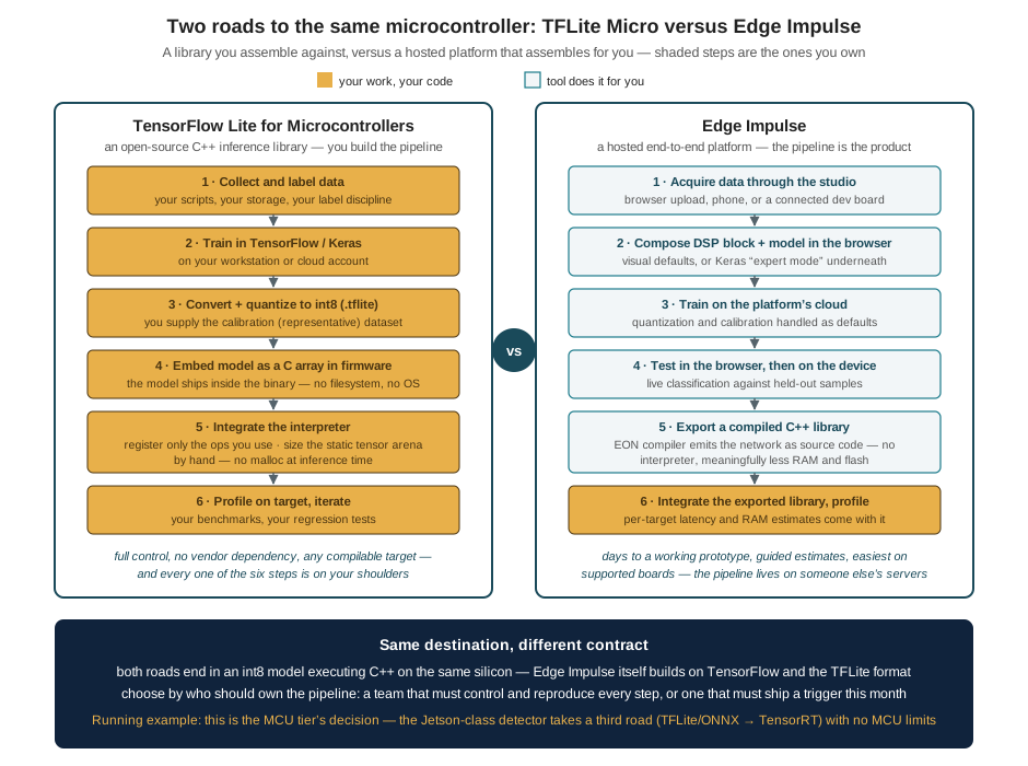
TensorFlow Lite for Microcontrollers is a library — an open-source C++ inference engine, a few tens of kilobytes compiled, designed for bare metal. It assumes nothing: no operating system, no filesystem, no dynamic allocation. The model arrives as a byte array compiled into the firmware; the developer instantiates an interpreter, registers only the operators the model actually uses (unused kernels never cost flash), and hands it a tensor arena — one statically allocated block, sized by hand through trial and profiling, from which every activation and scratch buffer is carved. Everything upstream of that integration — collecting data, training, converting, calibrating the quantization — is the developer’s own pipeline, in ordinary TensorFlow. The contract is maximal control and maximal responsibility: any target with a C++ toolchain, no vendor in the loop, and every one of the six pipeline stages on the team’s shoulders.
Edge Impulse is a platform — a hosted service in which the pipeline itself is the product. Data is acquired into a browser studio (uploaded, or streamed from a phone or a supported development board); a signal-processing block and a model are composed visually, with a Keras “expert mode” underneath for teams that outgrow the defaults; training runs on the platform’s cloud with quantization handled as a default; and the export is a compiled C++ library for the chosen target, with per-target latency and RAM estimates attached. Two details make it more than a convenience wrapper. Its DSP-block-first design reflects real MCU practice, where a feature extractor (a spectrogram, a filter bank) in front of a tiny network routinely beats a bigger network on raw samples. And its EON compiler emits the network as generated source code rather than a flatbuffer walked by an interpreter, saving meaningful RAM and flash on chips where both are counted in kilobytes. The contract is the mirror image of TFLM’s: a working prototype in days and guided resource estimates, in exchange for a pipeline that lives on someone else’s servers, is easiest on supported hardware, and yields deep customization reluctantly.
The choice between them is an engineering-situation question, not a quality ranking — the more so because the roads share pavement: Edge Impulse builds on TensorFlow and the TFLite model format, and both roads end in int8 C++ on the same silicon. A team that must own, reproduce, and audit every stage — a research group whose experiment is the pipeline, a product team with compliance obligations, a project targeting an unsupported chip — takes the library. A team whose scarce resource is embedded-ML engineering time — a field-robotics group that needs a vibration trigger working this month, a classroom, a prototype racing a funding deadline — takes the platform, and graduates to the library if and when its needs outgrow the defaults. For the running example, this entire comparison lives at the MCU tier — the always-on trigger of a cascade, should the system grow one. The goose detector itself, resident on the Jetson, takes the third road already described: trained in PyTorch, exported, quantized, and handed to TensorRT, with no MCU ceiling in sight.
That closes the frame this chapter opened. The placement hierarchy assigns the detector to the companion tier; the memory bill says what fitting there means; quantization and its siblings are how the fit is achieved; and the pipeline and its toolkits are how the result travels from a training run to a process consuming camera tensors inside the running example’s Detector node. What the frame still lacks is its center: the trained model itself — the dataset of geese and not-geese, the labeled boxes, the training runs and their failure modes. That is the next chapter, and it is where Part III stops preparing and starts building.
14.9 Check Your Understanding
- A detection head ends in a 1 × 1 convolution from 512 input channels to 21 output channels. Compute its weight count and its memory at float32 and at int8 (ignore biases). Per-channel quantization adds one float32 scale per output channel: compute the metadata overhead as a percentage of the int8 weight memory, and state why the overhead was negligible for the chapter’s 128-to-256-channel example but is less so here.
Weights: \(1 \times 1 \times 512 \times 21 = 10{,}752\). At float32: \(10{,}752 \times 4 = 43{,}008\) B ≈ 43 KB; at int8: 10,752 B ≈ 10.8 KB — the factor of four as always. Metadata: 21 scales × 4 B = 84 B, about 0.8 % of the int8 weights. The chapter’s example carried 256 scales against 294,912 int8 weights (≈ 0.35 %). The general rule: per-channel overhead is (4 B × output channels) against (1 B × weights per channel × channels), so it grows as layers get thinner — fewer weights per output channel. For very small layers the metadata fraction rises, which is one reason tiny models benefit proportionally less from quantization than their headline parameter counts suggest.
- Quantization does not reduce the number of multiply-accumulate operations a model performs, yet int8 inference commonly runs two to four times faster than float32 on the same embedded CPU. Give the two main mechanisms, and explain why the same reasoning predicts that quantization speeds up a memory-bound workload more than a compute-bound one.
First, memory traffic: embedded inference is usually limited by moving weights and activations through DRAM and cache, not by arithmetic; int8 quarters every operand, so the memory system delivers the same layer in a quarter of the bytes, and four times as much of the model stays cache-resident. Second, vector width: a SIMD unit is a fixed number of bits wide, so each instruction processes 4× as many int8 values as float32 values. Both mechanisms accelerate the supply and throughput of operands, not the operation count — so a workload already bottlenecked on memory gains nearly the full factor, while a compute-bound workload (small model, fast memory) gains only what wider integer SIMD provides. This is also why the energy saving tracks the speedup: the dominant energy cost is data movement, and quantization is a data-movement optimization.
- Assign each task to a tier of the compute hierarchy — cloud, companion computer, or MCU — and justify with the chapter’s criteria (latency, bandwidth, power, link reliability, privacy): (a) deciding, within one frame time, whether the deterrence target’s position has updated; (b) retraining the detector on last month’s hard cases; (c) monitoring motor vibration continuously for bearing wear, including while the main computer is under full perception load.
- Companion computer: the decision is consumed at frame rate by the control loop, so it cannot tolerate a radio’s variable latency or failure modes — the urgent path stays local, and only this tier has the GPU to run the detector. (b) Cloud: retraining is compute-hungry, deadline-free, and needs the accumulated dataset — exactly the “can wait” workload; only summaries and hard cases need to cross the link, and in batch. (c) MCU: an always-on 1-D classifier on accelerometer windows costs milliwatts and kilobytes, runs regardless of what the companion computer is doing (a key point — the Jetson under full perception load is exactly when a competing monitor would be starved), and needs only to raise a flag when something is anomalous. The pattern is the chapter’s cascade: cheap and always-on at the bottom, capable and framewise in the middle, heavy and offline at the top.
- Using the chapter’s accounting, estimate the RAM peak for the running example’s detector deployed as int8 with a 320 × 320 model input: weights 3.2 MB, peak activations 2.3 MB, a capture pipeline holding two 640 × 480 × 3 uint8 camera frames, and 1 MB of runtime workspace. Then explain why a further halving of the model input to 160 × 160 shrinks one term by four but two of the terms not at all — and which mission quantity, from the Images as Data chapter, the halving would damage.
Frames: \(2 \times 921{,}600 \approx 1.84\) MB. Peak ≈ \(3.2 + 2.3 + 1.84 + 1.0 \approx 8.3\) MB. Halving the input side to 160 × 160 divides activation memory (and per-frame compute) by four — activations scale with the model’s input pixel count — but the weights are fixed by the architecture, and the camera buffers are fixed by the sensor’s resolution, which does not change when the model’s input does. The damaged quantity is pixels on target: the Images as Data chapter showed the pixels a goose subtends scale with the model-input resolution the detector actually sees, so halving the input halves pixels-on-goose and with it the usable detection range — the resolution lever is always pulled against the mission’s geometry.
- Post-training quantization calibrates a layer’s activation scale from representative inputs. Suppose the calibration set for the goose detector was collected indoors, and a layer’s activations there span \([0, 6]\), so \(S\) is chosen as \(6/255 \approx 0.024\) — but in bright field conditions the same layer’s activations reach 24. What happens numerically to the flight-time activations, why does the damage not show up on the calibration data, and what does this imply about who should assemble the calibration set?
Every activation above 6 quantizes to \(q = 255\) and is clipped: the top three-quarters of the layer’s real dynamic range collapses onto a single level, so exactly the strong responses — the layer’s most confident feature detections — become indistinguishable from one another, and the layers downstream inherit saturated, information-poor inputs. On the calibration data the model is bit-for-bit healthy, because no calibration input ever exceeds the measured range; the failure is invisible until deployment conditions diverge from calibration conditions. The implication: the calibration set is mission data, not convenience data — it must span the lighting, altitude, and scene conditions of flight, which makes calibration a dataset-engineering task belonging to the same discipline (and the same chapter, the next one) as the training set itself.
- A university field-robotics group wants an acoustic trigger on a drone that wakes the main perception stack when it hears geese; one member has embedded experience, none has ML-pipeline experience, and the demonstration is in six weeks on a supported development board. A second group is building a certifiable agricultural product on a custom STM32 board and must reproduce every build from version-controlled sources. Recommend a toolkit for each, and state why neither recommendation applies to the goose detector itself.
First group: Edge Impulse — the constraint is embedded-ML engineering time, the board is supported, and the platform’s owned pipeline (acquisition, DSP block, training, compiled C++ export with resource estimates) converts six weeks into a plausible schedule; the DSP-first design suits an acoustic trigger particularly well. Second group: TensorFlow Lite for Microcontrollers — a custom board is outside any platform’s supported list, and certifiability demands that every pipeline stage (data, training, conversion, calibration, integration) be owned, version-controlled, and reproducible in-house, which is precisely the library’s contract. Neither applies to the goose detector because it runs on the companion tier, not an MCU: a Jetson-class board with gigabytes of RAM takes the TFLite/ONNX-to-TensorRT road, and the MCU toolkits’ defining constraints — kilobyte arenas, no OS, interpreter-free execution — are constraints it does not have.
14.10 Try It
Part 1 — quantize a real model and audit the damage. In a notebook, take any small trained vision model (a Keras MobileNet variant, or the small CNN you built for the previous chapter’s exercises) and walk it through post-training quantization with the TFLite converter: export it once as float32 and once as full-int8 with a calibration generator that yields a few hundred representative inputs. Compare the two files’ sizes on disk against this chapter’s factor-of-four prediction (and explain any shortfall — which parts of a .tflite file are not weights?). Then run both models over a held-out set and measure the damage directly: the maximum absolute difference in output scores, and the number of inputs on which the predicted class actually changes. Finally, sabotage the calibration deliberately — calibrate on a single image, or on blank frames — re-export, and watch the failure mode of Check question 5 appear in your own accuracy numbers.
Part 2 — itemize a memory bill. Using a model-summary tool (torchinfo in PyTorch, model.summary() in Keras), tabulate for the same model, layer by layer: parameter count, parameter bytes at float32 and int8, and output-activation bytes at float32 for a 640 × 640 input. Identify where the activation peak sits, and compare peak activations to total weights — then repeat at a 320 × 320 input and confirm the activations quarter while the weights do not move. Add realistic buffer terms (two camera frames at your sensor’s resolution, 1 MB of workspace) and produce your own version of this chapter’s memory-bill chart. Close with two sentences: one stating which single change most reduces your model’s RAM peak, and one stating what that change costs the mission, in the currency of the Images as Data chapter’s pixels-on-target arithmetic.
Related Lab: See Appendix B for the lab assignment that applies this chapter’s concepts.