17 Case Study: Wildlife Detection from the Air
Every quantitative claim in this Part so far has been the book’s own: worked miniatures, illustrative budgets, published benchmark tables read at a distance. That was the right way to build the machinery, but machinery built entirely from first principles carries a standing risk — that the problems it prepares for are not quite the problems the field actually has. The corrective is a case study, and this chapter conducts one. Its primary text is a real research paper: a team at a New Zealand university spent years trying to detect sheep from a drone at 80 m, built their own dataset because none existed, compared five detector architectures head to head, and published what worked, what failed, and how fast each ran (Sarwar et al. 2020). Around that paper sits a wider literature — cattle counted from quadrotors (Barbedo et al. 2020), seabird colonies censused by the tens of thousands (Hayes et al. 2021), waterfowl surveys that include Canada geese by name (Zhai et al. 2025) — and a smaller, sharper literature on the other side of the camera: field measurements of what geese do when a drone approaches them (Bech-Hansen et al. 2019).
Reading published work is a skill this book has not yet asked for, so the chapter models it. The questions an engineer puts to a paper are the ones Part III has spent four chapters making precise: What are the problem’s constants — altitude, target size in pixels, background? Where did the dataset come from, how big is it, and how was it split? What does the headline metric actually compute, and at what operating point? And what did the authors not do — which claims are measurements and which are projections? Asked of the sheep paper, those questions return a study that lands with almost uncanny precision on the running example’s own territory: small whitish blobs against pasture, a detector meant for the aircraft, precision and recall argued over in percentage points. Asked of the goose literature, they return the constants the running example will actually face — including one, set by the geese themselves, that no previous chapter has priced.
17.1 Learning Objectives
- Explain why animal detection from a moving aerial platform is harder than static-camera detection, naming the five recurring challenges — scale variation, background contrast, clustering, motion, and structural false positives — with a quantified example of each from the published literature.
- Summarize the sheep-detection study’s approach: the dataset it had to build, the five architectures it compared, why a centroid-based UNet with the weighted Hausdorff distance won on both accuracy and speed, and what each losing architecture’s failure mode was.
- Analyze a published paper’s evaluation with the detection-metric machinery of this Part: identify why a centroid detector reports F1 rather than mAP, read a precision–recall pair as an operating point, and distinguish measured results from projected ones.
- Situate the running example’s goose-detection problem in the aerial-wildlife literature, using reported waterfowl results to predict which conditions will be easy, which hard, and by roughly how much.
- Derive the altitude bind: combine pixels-on-target arithmetic with measured goose disturbance responses to show why detection range and disturbance-free approach conflict, and name the sensor-side levers that relax the conflict.
17.2 Key Vocabulary
- Onboard detection — running the detector on the aircraft’s own computer rather than on the ground or in the cloud; the deployment mode Part III has argued for throughout, and the stated (but not demonstrated) goal of the sheep study.
- Aerial survey — a systematic overflight flown to detect, count, or map animals over an area; the observational mode of wildlife work, where the deliverable is a census rather than an intervention.
- Scale variation — the change in a target’s apparent pixel size with altitude and terrain: the same animal spans a few pixels or tens of pixels depending on range, so a detector must either see all scales in training or have the scale pinned by flight discipline.
- Small-object detection — the regime in which targets span roughly twenty pixels or fewer, too few to exhibit the internal detail general-purpose detectors rely on; the regime every high-altitude animal detector lives in.
- Animal clustering — the tendency of animals to group until their bodies touch or overlap in the image, merging distinct individuals into one blob and defeating both segmentation and box-based non-maximum suppression; the dominant reported error source across species.
- Centroid annotation — a ground-truth label consisting of a single point at each object’s center rather than a bounding box; natural for counting tasks and for small, overlapping targets, at the cost of the box-based metric machinery.
- False negative (missed detection) — an animal present but not detected; in a survey it biases the count low, in the running example’s mission it leaves a goose undeterred.
- False positive (false alarm) — a detection with no animal behind it — a rock, a fence post, a shed roof; in a survey it biases the count high, in the running example’s mission it spends a flight leg harassing grass.
- Disturbance response — the measurable behavioral reaction of animals to an approaching aircraft, from raised-head vigilance to flushing (the whole flock taking flight); a function of altitude and approach distance that field studies quantify and flight plans must respect.
17.3 The Problem the Literature Keeps Meeting
Why is finding an animal from a drone hard, when finding a face in a phone photo is solved? A camera trap bolted to a tree answers by contrast. The trap’s viewpoint never changes; its scale is fixed, so a deer is always roughly the same size in pixels; and its background is the same background, every frame, so the oldest trick in computer vision — model the background, subtract it, and whatever remains is the animal — works. A drone forfeits all three properties at takeoff. Every frame arrives from a different pose and altitude, under a different lighting angle, over a different patch of ground, and the aerial-animal literature is, at bottom, the record of what that forfeiture costs. Five challenges recur across it — across cattle, seabirds, waterfowl, and sheep, across a decade of architectures — with a regularity that marks them as properties of the problem rather than of any one study. Figure 17.1 collects them.
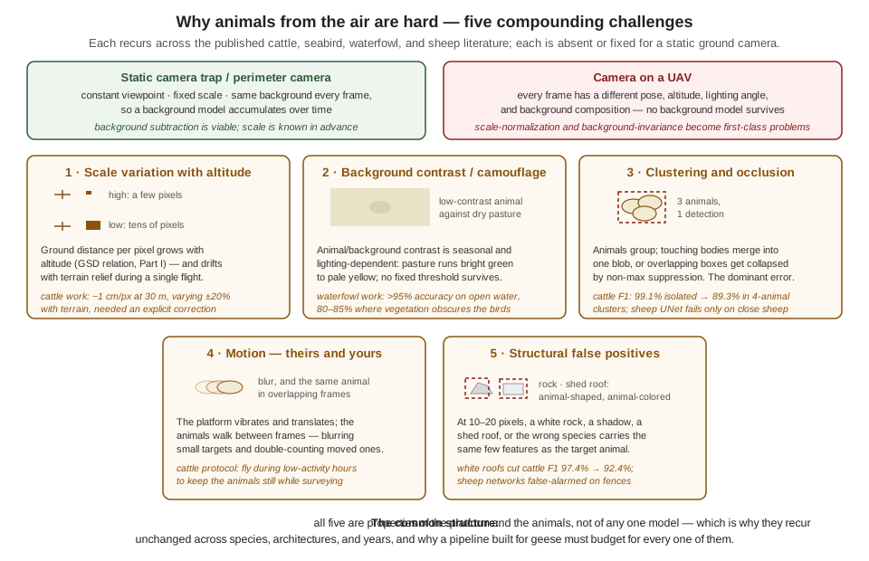
Three of the five deserve a sentence beyond the figure, because they will drive everything that follows. Scale variation is Part I’s ground-sample-distance relation acting as an adversary: a cattle-counting team reported a nominal 1 cm-per-pixel resolution at 30 m that wandered by ±20% with terrain relief alone, enough to break any size-based filtering until they built an explicit correction into the pipeline (Barbedo et al. 2020). Background contrast is not a fixed difficulty but a seasonal, lighting-dependent variable — the same team documented pasture ranging from bright green to pale yellow across a season — which is the field-scale version of the distribution-shift lesson the previous chapter drew, and it produces the single most consistent quantitative pattern in this literature: detection in the high 90s against simple backgrounds, dropping ten to twenty points wherever vegetation intrudes. And clustering is the failure that survives every architecture: animals bunch until their bodies touch, at which point a segmenter merges them, a box detector’s overlapping predictions get collapsed by the very non-maximum suppression step meant to clean duplicates — a seabird study watched legitimate penguin detections eliminated exactly this way (Hayes et al. 2021) — and a counting pipeline undercounts. Cattle F1 falls from 99.1% for isolated animals to 89.3% in four-animal clusters (Barbedo et al. 2020); geese, which raft together on water and graze in dense flocks, sit squarely in the danger zone.
The remaining two — motion, and structural false positives — round out the budget. Animals move between overlapping frames, so surveys double-count; the pragmatic mitigation in the cattle work is to fly when the animals are least active, a reminder that flight planning is part of the perception system. And at fifteen pixels, an animal is a shape and a color, which means everything sharing that shape and color is a candidate: white shed roofs depressed cattle F1 from 97.4% to 92.4% on the images containing them (Barbedo et al. 2020), rocks and shadows were logged as penguins (Hayes et al. 2021), and the sheep study’s own networks — the case this chapter now turns to — false-alarmed on fences.
17.4 Sheep at Eighty Metres
The sheep study’s problem statement is one sentence long and contains, on inspection, most of Part III. Detect sheep from a UAV flying at 80 m, where an adult sheep in a 2048 × 1080 video frame is “a rather nondescript whitish blob about 20 pixels long and 10 pixels wide” (Sarwar et al. 2020). Every number in that sentence is a decision. The altitude is a three-way compromise the authors state explicitly: 80 m — well under the 120 m legal ceiling that New Zealand shares with much of the world — bought enough detail on each sheep, enough paddock per frame to be useful, and minimal disturbance to the animals. The pixel count is that altitude passed through the pixels-on-target relation of the Images as Data chapter, and it is worth checking their arithmetic against ours, because the check teaches something. The platform was a consumer quadrotor whose camera family has a wide field of view of roughly 94°; spread over 2,048 columns that is about 0.8 mrad per pixel, so at 80 m each pixel covers about 6.5 cm of paddock, and a sheep roughly 1.2 m long by 0.6 m wide spans about 19 × 9 pixels — the paper’s 20 × 10, recovered from first principles. The same relation exposes the uncomfortable comparison: the running example’s depth camera in its 640-column mode subtends roughly 2.45 mrad per pixel, three times coarser, which is why its 0.35 m goose gets only 7 pixels at 20 m. The sheep team could fly at 80 m because their sensor spent 2,048 columns on the scene; angular resolution, not courage, sets the survey altitude.
Fifteen-ish pixels puts the task deep in small-object detection, and the paper’s literature review is a catalog of why that regime breaks the standard toolkit: small objects lack the internal detail — texture, parts, structure — that convolutional features feed on, and the authors note the YOLO family’s own documentation of its localization weakness on small targets, concluding that (as of the study’s writing) no off-the-shelf single-stage detector was good enough for the job (Sarwar et al. 2020). The claim has aged — the waterfowl literature below fields modern detectors against comparably small birds with strong results — but the underlying physics has not: a detector asked about a 15-pixel blob is reasoning from a few dozen informative values, and every design choice in the study flows from that scarcity.
The dataset had to be built, because — to the authors’ knowledge — no public dataset of drone imagery of sheep existed. This is the collect-and-label stage of the Building a Detection Pipeline chapter, executed for real, and the study’s choices read like that chapter’s checklist: video recorded at different times of day and in different weather, deliberately capturing the diversity of illumination, shadow, and background color; frames cut to 256 × 256 tiles; and, after augmentation, 22,742 labeled images split 80/10/10 into train, validation, and test. One labeling decision matters more than it first appears: every image was annotated twice, with bounding boxes and with centroid annotations — a point per sheep — because the five architectures under comparison consume different ground truth. The double labeling is the tell that this is a genuine comparison study: the same images, the same split, the same training budget, and only the detector varies.
17.5 Five Detectors, One Question
The comparison spans the two-stage/one-stage divide this Part has met twice already. On the two-stage side, the authors trained four networks through a modified R-CNN procedure — generate candidate regions, classify each — trimmed for the task: 1,000 region proposals per image instead of the classic 2,000, overlap thresholds tuned so that proposals count as positive examples more readily (small targets need every positive they can get), and a softmax-plus-cross-entropy classifier in place of the traditional support-vector-machine stage, purely to save training time. Two of the four were the era’s standard pretrained backbones, AlexNet and GoogLeNet, retrained on sheep. The other two were built for the occasion, and their design logic is the paper’s quiet thesis about small objects. Network-I is one convolutional layer, one fully connected layer, and a softmax — very nearly the smallest CNN that can exist — testing whether a tiny network suffices when the objects themselves carry so little detail. Network-II is seven convolution–batch-norm–ReLU–maxpool blocks that halve the spatial dimension at every step, 256 × 256 down to 2 × 2, deliberately densifying the features toward the end so that what survives is essentially the objects’ contour information — the authors’ explicit bet that a 15-pixel sheep is a contour and nothing else.
The one-stage entrant is the interesting one. Rather than YOLO or SSD — dismissed for their small-object record — the authors adopted a UNet: an encoder–decoder network with skip connections, producing not boxes but a full-resolution probability map, trained with the weighted Hausdorff distance as its loss (Sarwar et al. 2020). The ground truth here is the centroid labels, and the loss is built from the geometry of point sets — for estimated locations \(x\) with probabilities \(p_x\) and true centroids \(Y\):
\[ \begin{aligned} L_T(p, Y) \;=\;& \frac{1}{|X|+\varepsilon} \sum_{x \in \Omega} p_x \, \min_{y \in Y} d(x,y) \\ &+ \frac{1}{|Y|} \sum_{y \in Y} \min_{x \in \Omega} \frac{d(x,y)+\varepsilon}{\,p_x^{\alpha} + \varepsilon/d_{\max}\,} \\ &+ L_1\!\left(C - \hat{C}\right), \end{aligned} \]
whose two main terms are a conversation between prediction and truth: the first says everywhere you claim a sheep, a true centroid should be nearby — it penalizes confident probability mass far from any real sheep, which is the false-positive direction; the second says every true centroid should have confident probability mass nearby — it penalizes real sheep that no prediction approaches, the false-negative direction. The third term trains a count: a scalar regressed from the network’s deepest features, passed through a SoftPlus, \(\hat{C} = \log(1 + e^{s})\), and rounded to give the number of sheep directly. The architecture’s stated limitation is single-class operation — one species, no more, without modification — but for small, complexly shaped, overlapping objects, centroids have a structural advantage over boxes: two touching sheep have two distinct centers even when no line separates their pixels, and there is no non-maximum suppression step to collapse them.
All five networks trained under identical conditions — stochastic gradient descent, 500 epochs, on a single desktop GPU (an NVIDIA GTX 1080) — and the results are unambiguous:
| Network | Precision | Recall | F1-score | Location RMSE (px) | Time per image |
|---|---|---|---|---|---|
| UNet (centroids + WHD) | 96.20% | 90.14% | 93.07% | 0.783 | 0.14 s |
| Network-II (7-layer) | 91.21% | 81.91% | 86.31% | 1.819 | 2.22 s |
| Network-I (1-layer) | 88.77% | 80.45% | 84.38% | 1.961 | 0.20 s |
| GoogLeNet | 80.79% | 81.67% | 81.23% | 1.899 | 3.53 s |
| AlexNet | 78.74% | 81.37% | 80.03% | 2.132 | 1.31 s |
Figure 17.2 plots the table the way the previous chapter taught — accuracy against time — and the shape of the result is its own lesson. The previous chapter’s frontier forced a trade: more accuracy for more milliseconds, pick your point. Here there is no trade to make. The UNet wins every column at once — most accurate, fastest by a wide margin, tightest localization — because the four R-CNN-trained networks pay a structural tax it does not: a thousand region proposals per image, each classified separately, against the UNet’s single forward pass. Frontiers are properties of scaling within an architecture; across architectures, one design can simply dominate another for a given task, and finding the dominant design for this task — not the best-known design for tasks in general — is what the comparison bought.
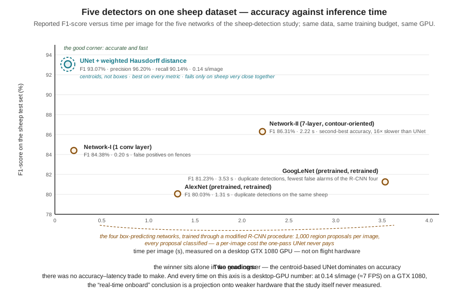
The failure modes are as instructive as the rankings, because they are the challenge taxonomy of Figure 17.1 reporting for duty. The two custom networks false-alarmed on fences — linear, high-contrast structures that share edge statistics with a sheep’s contour: structural false positives, exactly as the cattle and seabird studies predicted. The two pretrained backbones produced duplicate detections on the same sheep — several boxes on one animal — the pathology the detection-pipeline chapter’s matching rules would score as one true positive plus a string of false positives. And the winning UNet’s only reported failure is that it errs “when sheep are very close together” (Sarwar et al. 2020) — clustering, the challenge that survives even the architecture built to resist it. The best detector in the study fails exactly where the whole literature fails, which is the strongest evidence the chapter has that the taxonomy is real.
17.6 Reading the Results with Part III’s Instruments
Now put the paper under this Part’s instruments, starting with a question a careful reader should already have: where is mAP? The Building a Detection Pipeline chapter presented mean average precision as the standard detector summary, yet this study reports precision, recall, and F1 at a single operating point, and never mentions it. The answer is structural, and it generalizes. The entire mAP construction stands on IoU — box-overlap matching between prediction and ground truth — and the winning network has no boxes: a centroid detector’s output is a set of points, so matching must be by distance (is there a predicted point near enough to this true centroid?), localization quality becomes the root-mean-square error of matched locations — the table’s RMSE column, under one pixel for the UNet — and the natural summary becomes the precision/recall/F1 triple computed at the model’s operating point. The lesson is not that the paper is deficient; it is that the metric follows the output representation, and an engineer comparing this study against a box-detector paper must down-convert both to the common currency — TP, FP, FN — before believing any comparison. The counts, and the two ways of being wrong they encode, survive every change of representation; the summary statistics on top of them do not.
The operating point itself repays reading. Precision 96.2%, recall 90.1%: when this detector says sheep, it is right 24 times in 25, and it finds nine sheep in ten. That asymmetry — precision comfortably above recall — is well suited to the study’s implicit mission, which is counting: false positives corrupt a census as badly as false negatives, and a follow-up count-regression head makes systematic over-detection actively harmful. The running example’s mission prices the same two errors differently, as the detection-pipeline chapter argued: an unharassed goose is a mission failure, an investigated patch of empty grass a battery expense, so the goose detector deliberately trades precision for recall. Same machinery, opposite operating point — chosen, in both cases, in mission currency. A survey counts; a deterrence system must not miss.
Then there is the claim in the title, and the word doing quiet work in it: towards detection of sheep onboard a UAV. Nothing in the paper runs on an aircraft. Every timing in Table 17.1 was measured on a desktop GTX 1080; the onboard argument is a closing projection — the UNet’s 0.14 s per image, about 7 FPS, is fast enough that the authors are “confident” the task could run in real or near-real time on an embedded board such as the Jetson Nano, whose specifications (128 CUDA cores, 4 GB of shared memory, 5 W) they cite (Sarwar et al. 2020). The previous chapter equips the reader to see precisely what stands between that confidence and a flight: a Jetson Nano is not a GTX 1080 with fewer fins — it is an order-of-magnitude step down in cores, memory bandwidth, and power, sharing its memory with an operating system and (on a real aircraft) a full sensing stack. The measure-on-the-target discipline, the tail-latency question, thermal behavior under sustained load, the capture-and-preprocess stages that the 0.14 s figure does not include — every honest-benchmarking rule of the Real-Time Inference chapter names a gap between this paper’s last section and a working onboard system. None of this is a criticism of the study, which claims exactly what it demonstrates and flags the rest as future work; the same group’s journal follow-up reports a refined multi-scale U-Net variant reaching approximately 98% F1 on the sheep task (Sarwar et al. 2021). It is, rather, a calibration for reading: a paper’s conclusions section is where measurement ends and projection begins, and the reader is responsible for knowing which side of that line each claim lives on. The gap between “towards onboard” and onboard is, not coincidentally, the exact territory the previous two chapters of this Part were written to cross.
17.7 From Sheep to Geese
How hard is the running example’s problem, relative to the case just studied? The cross-species literature gives a calibrated answer, and Figure 17.3 assembles it. White sheep on green pasture sit near the easy pole of aerial animal detection — the highest animal-background contrast the problem ever offers, no vegetation tall enough to occlude, modest flock densities in the imagery. Geese offer none of those mercies, and the waterfowl literature quantifies what their absence costs. The most directly on-point study is a drone-based waterfowl survey system whose detection classes include Canada, Brant, and Emperor geese by name: it reports detection accuracy above 95% for birds sitting on open water — a background as clean as pasture — falling to 80–85% in vegetated and cropped habitat where birds overlap with cover (Zhai et al. 2025). That ten-to-fifteen-point drop is the background-contrast challenge measured on geese, and it forecasts the running example’s own validation table: strong over mown grass, weakest exactly where geese actually loiter — pond margins, reed beds, crop stubble.
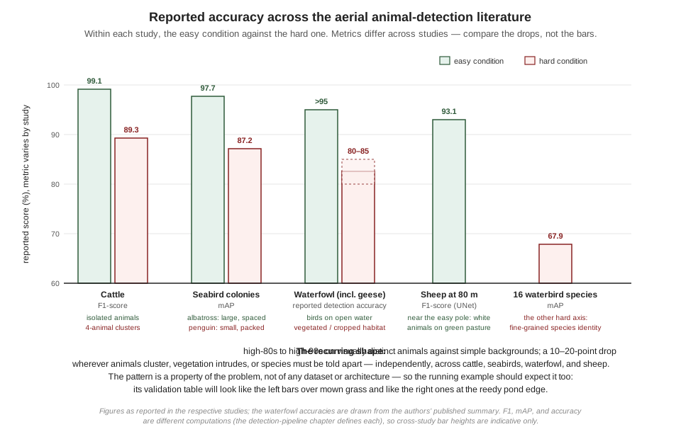
Two more bars on that figure locate the goose problem’s other axes. Where the task is a single visually distinct species against varied backgrounds, modern box detectors do well: a predecessor waterfowl effort — from the group behind the goose-inclusive survey system — assembled aerial duck datasets running to roughly 197,000 annotations and reported a Faster R-CNN baseline at 95.38% mAP (Zhang et al. 2022). Where the task becomes fine-grained — sixteen visually similar waterbird species on the Texas coast — reported mAP falls to 67.9% for the best model in a Faster R-CNN-versus-RetinaNet comparison (Kabra et al. 2022). The running example lives between those poles: two classes, goose and other_bird, which is fine-grained enough to be non-trivial (a distant duck and a distant goose are a few dozen pixels of brown each) but far from a sixteen-way identification. And on the sensing side, the literature has an answer the running example’s current payload does not exploit: for warm-bodied animals against cool backgrounds, thermal imaging substantially outperforms visible light alone — a wildlife-detection benchmarking effort reports large gains from thermal and fused streams over RGB (Chang et al. 2023) — and an open-source waterfowl identification tool built for management agencies pairs a thermal and an RGB sensor precisely to get detection from one and species identity from the other (Loken et al. 2025). Thermal is a payload and cost decision, not a free upgrade, but it is the standard escape hatch when visible-light contrast runs out — dusk, dawn, and vegetation — and worth holding in reserve against the robustness failure modes the previous chapter cataloged.
One more contrast between the sheep study and the goose problem is about time, and it is good news. The sheep team’s first act was building a dataset from nothing, because in their sub-field nothing public existed. The waterfowl sub-field, a few years on, is different: the goose-inclusive survey work publishes a companion dataset — reported at some nine thousand high-resolution aerial images carrying over half a million machine-assisted box annotations, Brant and Canada and Emperor geese among the classes, hosted in an open conservation-imagery repository (Zhai et al. 2025). For the running example’s collect stage, that changes the opening move the detection-pipeline chapter prescribed: public aerial goose imagery now exists at a scale no field campaign will match, ideal for pretraining and for populating the easy conditions — with the usual caveat that a dataset collected over an Alaskan lagoon shares neither the altitude profile, the optics, nor the backgrounds of the running example’s protected field, so the session-split discipline and the fly-your-own-camera collection round remain exactly as necessary as that chapter argued.
17.8 The Altitude the Animals Set
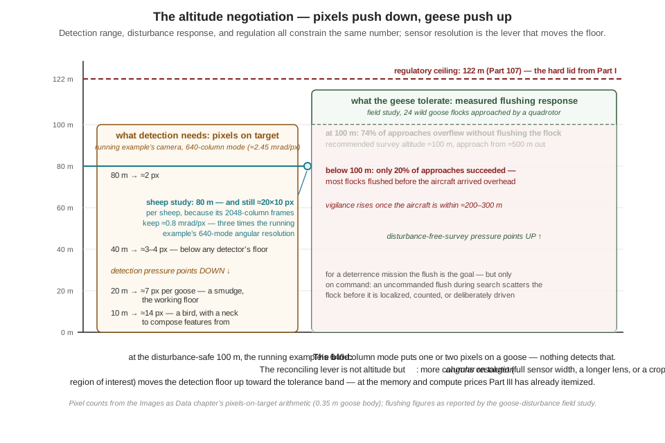
Every constraint on flight altitude so far in this book has come from physics or law: pixels-on-target from below, the 122 m ceiling from above, battery and coverage in between. The wildlife literature adds a constraint from an unexpected authority — the animals — and for geese specifically, it has been measured. A field study flew a consumer quadrotor toward 24 wild goose flocks of five species, at 50 m and 100 m altitude, and recorded the birds’ response (Bech-Hansen et al. 2019). The results draw a sharp line in the sky: approaches at 100 m overflew the flock without flushing it 74% of the time, while approaches below 100 m succeeded only 20% of the time — four flights in five, the flock was airborne before the aircraft arrived. Vigilance behavior began when the drone was still 200–300 m away, and the authors’ operational recommendation is blunt: to survey geese without disturbing them, launch about 500 m out and fly at about 100 m.
Set that finding against the pixels-on-target arithmetic and the bind is immediate. At the disturbance-safe altitude, with the running example’s camera in its 640-column mode,
\[ \begin{aligned} \text{metres per pixel at } 100\ \text{m} &= R\,\theta_{\text{pix}} = 100 \times 2.45 \times 10^{-3} = 24.5\ \text{cm} \\ \text{pixels on a } 0.35\ \text{m goose} &= \frac{0.35}{0.245} \approx 1.4\ \text{pixels}. \end{aligned} \]
One and a half pixels is not a small target; it is no target at all. The altitude band the geese tolerate and the altitude band the detector needs do not overlap — for this sensor configuration — and Figure 17.4 draws the squeeze. The sheep study threaded the same needle without remarking on it: 80 m was gentle enough for sheep (a species far more drone-tolerant than wild geese) while its 2,048-column sensor still delivered 20-pixel animals. The general lesson is the one the figure’s footer states: the reconciling lever is angular resolution, not altitude. Feeding the detector from the camera’s full sensor width rather than the reduced mode, cropping a full-resolution region of interest around a candidate before classifying it — the Images as Data chapter’s trick — or carrying a longer lens all raise the detection floor toward the tolerance band, each at memory, compute, and field-of-view prices this Part has already taught the reader to itemize.
A deterrence mission complicates the picture in an interesting way: flushing the flock is not a failure mode, it is the deliverable. But it is the deliverable on command — an uncommanded flush, triggered by the search pattern itself, scatters the flock before it has been localized and before the system can drive it in a chosen direction, and it habituates the birds to exactly the stimulus the mission depends on. Disturbance, in other words, is a resource to be spent deliberately, not leaked; and the broader literature on drone disturbance of wildlife — now substantial enough to support systematic review (Afridi et al. 2025) — is the reference the mission’s ethics chapter in Part V will draw on when it prices that spending properly. The nearest thing the published record offers to the running example as a whole system is instructive to name here: a field-tested agricultural drone that detects deer with a YOLO-family model, plans coverage paths over the protected crop, and returns to an autonomous charging station between sorties (Temesgen et al. 2025) — detection, planning, and endurance engineering composed into one loop. That composition — what the detector node publishes, who consumes it, and how the mission logic, planner, and platform close around it — is precisely the subject the System Architecture chapter of Part V takes up for the running example itself.
17.9 What the Case Study Settles
Six findings travel from this chapter’s reading directly into the running example’s design file. First, the challenge taxonomy is real: scale variation, background contrast, clustering, motion, and structural false positives recur, quantified, across every species and architecture surveyed, so a goose pipeline budgets for all five or rediscovers them in the field. Second, the small-object regime governs architecture: below about twenty pixels, standard detectors weaken and task-shaped designs — up to and including abandoning boxes for centroids — can dominate the general-purpose toolkit on accuracy and speed at once. Third, the metric follows the output representation, and comparisons across papers are made in the common currency of TP, FP, and FN, at stated operating points, or not at all. Fourth, easy and hard conditions differ by ten to twenty points everywhere in this literature; the running example should plan for that spread — per-condition evaluation, targeted collection at the reedy margins — rather than be surprised by it. Fifth, “towards onboard” and onboard are separated by exactly the disciplines of the previous two chapters: target-hardware measurement, latency budgets, and the quantize-convert-deploy pipeline; a desktop-GPU timing is the beginning of that argument, never its end. And sixth, the animals are a stakeholder in the flight plan: measured disturbance responses set an altitude band as binding as any regulation, and reconciling it with pixels-on-target is a sensor-resolution problem the design must solve on purpose.
The Part’s story is now complete twice over — once as machinery, built across four chapters, and once as corroboration, read out of the published record of people solving the same problem for sheep, cattle, seabirds, and geese. What remains is everything the detector’s output feeds: the search patterns that put the camera over the right field, the pursuit behaviors that spend the detections, and the coordination that makes several aircraft more than the sum of their cameras. That is Part IV’s territory.
17.10 Check Your Understanding
- The sheep study reports its animals as roughly 20 × 10 pixels at 80 m, while the running example’s goose spans only about 7 pixels at 20 m — four times closer, yet fewer pixels. Reconstruct the arithmetic that explains the apparent paradox, and state the general design lesson.
Pixels on target depend on range and per-pixel angle: pixels ≈ (target size)/(R·θpix). The sheep platform spreads a ~94° field of view over 2,048 columns, giving θpix ≈ 0.8 mrad, so at 80 m each pixel covers ~6.5 cm and a 1.2 m sheep spans ~19 pixels. The running example’s 640-column mode spreads ~90° over 640 columns — θpix ≈ 2.45 mrad, three times coarser — so at 20 m each pixel covers ~4.9 cm and a 0.35 m goose spans ~7. The sheep is also simply a bigger animal. Lesson: angular resolution (sensor columns per degree) is as decisive as altitude, and it is a design variable — full-sensor capture, region-of-interest crops, or a longer lens buy detection range without descending.
- The sheep study never reports mAP, the metric the detection-pipeline chapter called the standard detector summary. Explain the structural reason, name what the study reports instead for localization quality, and state the rule for comparing its results against a box-detector paper’s mAP.
mAP is built on IoU matching, and IoU requires boxes; the winning UNet predicts centroids — points — so box overlap is undefined. Matching must instead be by distance (a predicted point close enough to a true centroid is a TP), and localization quality is reported as the RMSE of matched locations (0.783 px for the UNet). Precision, recall, and F1 survive unchanged because they are computed from TP/FP/FN counts, which any matching rule produces. The comparison rule: reduce both papers to counts and stated operating points before comparing — F1 at one threshold and mAP (an area over all thresholds) are not directly comparable numbers, and the matching criteria beneath them differ besides.
- The sheep detector operates at precision 96.2%, recall 90.1%; the detection-pipeline chapter argued the goose detector should operate with recall above precision. Explain why both choices are correct, in the currency each mission uses.
The operating point prices the two error types against mission costs. The sheep system’s implicit mission is counting: a false positive inflates the census exactly as a false negative deflates it, and the paper’s count-regression head makes systematic over-detection actively corrupting — so precision is kept high, accepting that one sheep in ten is missed in any single frame. The goose mission is deterrence: a false negative is a goose left undeterred (the mission’s purpose unmet), while a false positive costs battery and time investigating grass — so the threshold moves down, trading precision for recall. Same machinery, opposite corners: the confidence threshold belongs to the mission, not the model.
- The winning UNet’s only reported failure is on sheep “very close together” — and clustering is also the dominant reported error for cattle, penguins, and vegetated waterfowl. Explain why clustering defeats box detectors and centroid detectors through different mechanisms, and name the machinery from the Real-Time Inference chapter that partially compensates in the running example.
Box detectors on clustered animals produce heavily overlapping predictions, and non-maximum suppression — the step that removes duplicate boxes on one object — cannot distinguish “two boxes, one animal” from “two boxes, two touching animals,” so it collapses legitimate detections (the seabird study’s penguin failure). Centroid detectors avoid NMS but fail when the probability map’s peaks merge: two animals close enough that their predicted probability mass fuses into one blob yield one centroid. Both mechanisms undercount. In the running example, tracking helps at the margins: animals that separate even briefly across frames get distinct track identities that persistence and coasting can maintain through subsequent merges — though a flock that never separates remains undercounted, which is one reason flock-level behavior (Part IV) matters more than per-bird counts for deterrence.
- The sheep paper concludes that detection “should be able” to run in real or near-real time onboard, citing the UNet’s 0.14 s per image and the Jetson Nano’s specifications. Using the previous chapter’s disciplines, list what this projection has not yet established, and estimate the first-order concern.
The 0.14 s (~7 FPS) was measured on a desktop GTX 1080; the projection target is an order of magnitude weaker in cores, memory bandwidth, and power. Unestablished: (1) on-target latency — measured on the Nano, not inferred from spec sheets; (2) the full budget — 0.14 s covers inference, not capture, preprocessing, or postprocessing; (3) tail latency, not just a mean; (4) sustained thermal behavior at 5–10 W in an enclosure; (5) contention with the rest of a flight stack sharing the same memory and cores. First-order concern: raw throughput — a conservative scaling of a 0.14 s desktop-GPU inference onto Nano-class hardware lands at whole seconds per frame, far from frame rate, which is why the deployment chapters’ quantization, resolution, and runtime-optimization levers (int8, TensorRT) are not optional refinements but the difference between the projection and a working system.
- The goose-inclusive waterfowl study reports >95% detection accuracy on open water but 80–85% in vegetated habitat. Restate this result in the vocabulary of the previous chapter’s robustness section, and derive from it two concrete rows in the running example’s evaluation plan.
It is a quantified, condition-dependent performance gap: background composition is a dimension of the input distribution, and pooled accuracy hides a ten-to-fifteen-point spread between its easy and hard regions — exactly the argument for per-condition evaluation rather than one averaged number. Evaluation-plan rows: (1) report the goose detector’s metrics separately for open-ground/open-water backgrounds versus vegetated-margin backgrounds (reed beds, pond edges, crop stubble), so the gap is measured before deployment rather than discovered during it; (2) weight the next collection round toward the hard condition — vegetated-margin footage with partially occluded geese, labeled under the written class-boundary rules for partial visibility — since that is where both the literature and the mission’s geese concentrate the failures.
17.11 Try It
Part 1 — read a paper with the instruments. Choose one study from this chapter’s literature — the cattle, seabird, waterfowl, or multi-species waterbird paper — and extract it into a one-page engineering brief using this chapter’s template: the problem’s constants (altitude or GSD, target size in pixels, background types); the dataset (source, size, annotation type, split discipline — and whether the split would pass the detection-pipeline chapter’s leakage test); the method (architecture, one-stage or two-stage, loss, ground-truth representation); the evaluation (which metrics, at what operating point or threshold, and what the matching criterion was); and the claims ledger — two columns, measured versus projected, with every conclusion in the paper assigned to one. Close with three sentences: the result most transferable to the goose problem, the result least transferable and why, and the one experiment you would run that the authors did not.
Part 2 — reproduce the small-object cliff. Take the detector you fine-tuned in the detection-pipeline chapter’s exercise and measure how its accuracy degrades as targets shrink toward the sheep paper’s regime. Downsample your validation images by factors of 2 and 4 (then upsample back to the model’s input size, so input resolution is constant and only target scale changes — this simulates flying 2× and 4× higher), and run validation at each scale. Plot mAP@0.5 against median target size in pixels, and find your detector’s cliff — the target size at which mAP falls below half its full-scale value. Compare your cliff against the pixels-on-target table for your own camera: what is the maximum altitude at which your detector’s targets stay above the cliff? Finally, test one mitigation from this chapter: crop full-resolution regions of interest around targets in the downsampled-by-4 condition and re-run validation on the crops — and report, in two sentences, how much of the lost accuracy the resolution lever recovered and what the crop cost you in field of view.
Related Lab: See Appendix B for the lab assignment that applies this chapter’s concepts.