27 Remote Sensing at Scale: Multispectral Imaging in Agriculture
The previous chapter closed on a debt no log can pay — whether a flight should have happened at all is an account this Part renders in its final chapter — but before it does, an older promissory note from Part I falls due. The Commercial Drone Landscape chapter, surveying the agricultural vertical, introduced the multispectral camera and the normalized difference vegetation index, showed a real NDVI field map, and explained why the measurement is harder than the formula suggests — then explicitly deferred the hard part, promising that this chapter would develop multispectral radiometry, calibration, and index construction in full. This chapter pays that debt, and in paying it does something the book has not done since Part I: it steps outside the running example’s sensing paradigm entirely. Nearly every perception page since Part III has been about finding discrete objects — a goose, a bounding box, a confidence score — in single RGB frames. Agricultural remote sensing is the commercial drone world’s other great sensing paradigm, and it works nothing like that: no object detector, no bounding box, no target class. It is a per-pixel physical measurement, assembled across a whole field, whose “detection” is a spatial anomaly in a continuous index — and whose most interesting modern frontier is squeezing a diagnosis, not just an alarm, out of the spectrum.
That frontier is where this chapter spends its depth, because the foundation is already laid. The Commercial Drone Landscape chapter established what NDVI is, which five bands a standard agricultural multispectral array carries, why healthy vegetation reflects near-infrared strongly, and how index maps become prescription maps; none of that is repeated here. What Part I’s treatment deliberately left general is the question this chapter makes specific: NDVI’s spatial variation “reveals stress — drought, nutrient deficiency, disease, pest damage,” all lumped together. A depressed index says something is wrong. It does not say what. Telling a fungal infection apart from a dry week is a genuinely different problem — one the plant-pathology remote-sensing literature attacks with purpose-built red-edge indices and per-disease classifiers, with real head-to-head numbers against NDVI — and it comes packaged with an operational question the book is unusually well equipped to answer: how a sensing mission is actually flown, coarse survey first, targeted re-fly on what the survey flags, using precisely the coverage-pattern machinery the Path Planning on the Edge chapter built for the running example’s search grid.
27.1 Learning Objectives
- Carry a multispectral image from raw digital numbers to calibrated surface reflectance — downwelling irradiance sensor, reflectance panel, solar-noon flight window — and explain why vegetation indices are computed from reflectance rather than pixel brightness, completing the radiometry the Commercial Drone Landscape chapter deferred to this chapter.
- Explain why generic NDVI is a good stress detector but a poor stress classifier, and describe the red-edge mechanism — chlorophyll breakdown and cell-structure disruption in fungally colonized tissue — that disease-specific indices exploit and NDVI’s broad red/NIR contrast largely misses.
- Compute NDRE and REDSI from band reflectances, and interpret REDSI’s published head-to-head accuracy against NDVI on wheat yellow rust, including what the validation platform does and does not license you to claim.
- Summarize two real UAV disease-detection case studies — sugar beet Cercospora/powdery mildew and wheat stem rust — with their actual platforms, ground sample distances, classifiers, and per-class accuracies, and present early-detection lead times as a disease-specific range rather than one universal number.
- Design a coarse-to-targeted two-stage crop-scouting survey: parameterize the Path Planning on the Edge chapter’s lawnmower generator for each stage, work the GSD-versus-track-length arithmetic that motivates the split, and state when adaptive sampling beats exhaustive coverage.
- Contrast per-pixel continuous-index sensing with Part III’s per-frame discrete object detection precisely — same sensor category, different information-processing problem — and identify which paradigm, or which hybrid, a given sensing task calls for.
27.2 Key Vocabulary
- Radiometric calibration — the conversion of a camera’s raw digital numbers into surface reflectance: a downwelling irradiance sensor records the illumination striking the scene, a panel of known reflectance imaged on the ground anchors the scale, and the ratio of reflected to incident light becomes a property of the plant rather than of the weather.
- Red edge — the steep transition in vegetation reflectance between strong chlorophyll absorption in the red and strong leaf-structure scattering in the near-infrared, roughly 700–740 nm; its position and slope shift with chlorophyll content and cell condition, which makes it the recurring diagnostic region for crop disease.
- Spectral signature (disease-specific sense) — beyond Part I’s general notion of a surface’s reflectance-versus-wavelength shape: the characteristic perturbation a particular stressor imposes on that shape — a fungal infection raising visible and red-edge reflectance while lowering NIR is a different signature from drought’s flatter, NIR-dominated depression, even when both depress NDVI equally.
- NDRE (Normalized Difference Red Edge) — the normalized-difference index formed from NIR and red-edge reflectance, \((\rho_{\text{NIR}} - \rho_{\text{RE}})/(\rho_{\text{NIR}} + \rho_{\text{RE}})\); identical in form to Part I’s NDVI with the red band swapped for the red-edge band, less prone to saturating over dense canopy and more sensitive to early chlorophyll loss.
- REDSI (Red Edge Disease Stress Index) — a purpose-built disease index computed from red and two red-edge bands, designed around the specific way wheat yellow rust distorts the red-edge region; the index with the clearest published head-to-head win over NDVI on the same plots.
- Hyperspectral imaging — imaging in hundreds of contiguous narrow bands (a few nanometres each) rather than a handful of discrete filtered bands, so each pixel carries an essentially continuous spectrum; heavier, costlier, and hungrier for calibration than multispectral, but able to resolve diagnostic wavelengths a five-band filter set was not designed to isolate.
- Coarse-to-targeted search (two-stage survey) — the crop-scouting flight doctrine in which a first pass covers the whole field at high altitude and coarse GSD to build an index map, anomalous sectors are flagged algorithmically, and a second pass re-flies only the flagged sectors at low altitude and fine GSD to confirm and diagnose.
- Ground sample distance (GSD) — Part I’s centimetres-per-pixel measure, reappearing here as the two-stage survey’s control variable: the Commercial Drone Landscape chapter’s relation makes it linear in altitude, so each stage’s altitude choice is a resolution choice, and the coarse and targeted stages are two points on the same line.
27.3 The Measurement Beneath the Index
Part I flagged the problem in one sentence — reflectance is a ratio of reflected to incident radiance, and the incident term varies with sun angle, cloud, and haze between one flight line and the next — and this section discharges it, because every index in this chapter is meaningless without it. What a camera pixel records is a digital number proportional to the radiance entering the lens, which is the product of two things: how strongly the surface reflects at that band, and how much light was falling on it at that moment. Only the first factor is about the plant. A cloud shadow crossing the field mid-flight can depress raw NIR brightness by more than a diseased canopy does; a survey stitched from frames taken twenty minutes apart bakes the sun’s motion into the mosaic. An index computed from raw digital numbers is therefore an index of the weather as much as of the crop.
The field workflow that removes the illumination term has three standard parts, and agricultural multispectral rigs ship with the hardware for the first two. A downwelling irradiance sensor — an upward-facing light meter, filtered to the same bands as the camera — rides on top of the aircraft and logs incident illumination for every exposure, so each frame’s radiance can be divided by the illumination that produced it. A calibrated reflectance panel — a target of known, spectrally flat reflectance — is imaged on the ground before and after the flight, anchoring the ratio to an absolute scale: if the panel reflects 50 % by manufacture and reads a given digital number, the scale factor from number to reflectance follows for every band. And the flight window is scheduled near solar noon on a stable sky, not for convenience but because both corrections are approximations — the irradiance sensor measures illumination at the aircraft, not in the crop’s shadowed lower canopy, and the panel calibration holds only while the atmosphere resembles the moment it was imaged. Photogrammetry software then assembles the calibrated frames into the orthomosaic Part I defined, using generous overlap between frames so that every point on the ground is imaged several times and the stitcher has features to match; the sugar-beet study worked through below flew 80 % front and 70 % side overlap, which is representative (Koç et al. 2025).
Why go to this trouble when the index is a ratio anyway? Normalized-difference indices do cancel some illumination variation — a uniform brightening multiplies numerator and denominator alike — and that partial self-correction is a real reason the form is popular. But the cancellation is only exact if illumination shifts identically in both bands, and it does not: haze scatters blue and red far more than NIR, and canopy shadow is not spectrally neutral. The indices this chapter cares about are also being asked a harder question than Part I’s. Distinguishing a diseased pixel from a merely dry one turns on reflectance differences of a few percentage points in a 35-nanometre-wide band; that signal does not survive an uncalibrated pipeline. Calibration discipline is to this chapter what cross-track error was to the Path Planning on the Edge chapter — the unglamorous budget line the whole guarantee rests on.
27.4 A Detector Is Not a Classifier
With calibrated reflectance in hand, Part I’s story can be sharpened into this chapter’s central distinction. NDVI works as a stress detector because nearly every way a plant can suffer eventually erodes the same contrast: less photosynthetically active tissue means less red absorption and less NIR scattering, so the index falls. That convergence is exactly what makes NDVI a poor classifier — drought, nitrogen shortage, a fungal colony, and chewing insects all arrive at the same depressed number by different routes, and by construction the index has thrown away the route. Two bands in, one scalar out: everything the spectrum knew about which stressor is at work was discarded at the moment of the subtraction.
The information NDVI discards is concentrated in a region NDVI does not sample. Between the red band’s deep chlorophyll absorption and the NIR plateau’s structural scattering lies the red edge, the steep shoulder around 700–740 nm where vegetation reflectance climbs by an order of magnitude in a few tens of nanometres. The shoulder’s position and slope are set by the two things a fungal infection attacks first: chlorophyll concentration, which the pathogen degrades as it colonizes leaf tissue, and cell structure, which collapses as mycelium spreads and pustules erupt. Both changes move and flatten the red edge before the broadband red/NIR contrast has fully deteriorated — which is the physiological reason spectral methods can beat a human scout, since the reflectance change precedes the visible pigment loss an eye detects. And the perturbation is not the same for every stressor. A multi-temporal vineyard trial in Portugal’s Vinho Verde region that tracked downy mildew across seven multispectral flights over treated and untreated vines reported the infection signature as increased reflectance in the visible and red-edge bands with a progressive decline in NIR — an opposite-signed, two-part pattern distinguishable from the flatter, NIR-dominated depression of simple water stress (Unknown (full author list not retrieved) 2025). Work on potato late blight makes the mechanism finer still: infection measurably shifts the wavelength positions of two spectral landmarks — the red-well point, where red absorption bottoms out, and the red-edge point, where the shoulder’s slope peaks — and a classifier watching those red and red-edge wavelengths reached 89.3 % accuracy at leaf scale three days after inoculation, the same day symptoms first became visible, and 89.1 % at canopy scale two days later (Fernández et al. 2020).
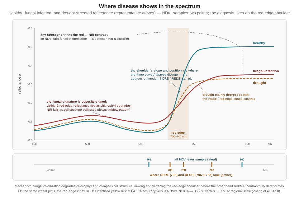
Figure 27.1 draws the argument. The two teal markers under the wavelength axis are all NDVI ever sees; every curve in the figure loses contrast between them, which is why the index detects them all and distinguishes none. The amber markers sit on the shoulder, where the curves’ shapes diverge. An index built from those bands is not more sensitive in some vague sense — it is sampling the specific spectral degrees of freedom that carry the disease information. The next section builds two such indices and puts real accuracy numbers behind the claim.
27.5 Indices Built for Diagnosis
The gentlest step beyond NDVI keeps the normalized-difference form and moves one band. NDRE replaces red with red-edge:
\[ \text{NDRE} = \frac{\rho_{\text{NIR}} - \rho_{\text{RE}}}{\rho_{\text{NIR}} + \rho_{\text{RE}}}, \]
computable on any standard five-band agricultural array, since the array carries a red-edge filter precisely for indices like this one. Because red-edge reflectance — unlike deep-red reflectance, which is nearly zero for any healthy canopy — still varies with chlorophyll content in dense vegetation, NDRE keeps discriminating after NDVI has saturated over a closed canopy, and it responds to early chlorosis while the red band is still pinned near total absorption. The same one-band substitution logic produced GNDVI, the green-for-red variant introduced for chlorophyll and nitrogen estimation (Gitelson, Kaufman, and Merzlyak 1996), which reappears throughout the disease literature because disease-driven chlorophyll loss is exactly what it was built to sense.
The sharper instrument is an index designed around one disease’s signature. The Red Edge Disease Stress Index was constructed from the specific way yellow rust — the fungal disease Puccinia striiformis causes in wheat — distorts the red-edge region, and it uses three bands: red at 665 nm and two red-edge bands near 705 and 783 nm (Zheng et al. 2018):
\[ \text{REDSI} = \frac{(705-665)\,(\rho_{\text{RE3}} - \rho_{R}) \;-\; (783-665)\,(\rho_{\text{RE1}} - \rho_{R})}{2\,\rho_{R}}. \]
The construction is a triangle: the numerator measures how far the mid-shoulder reflectance sits from the straight line joining the red trough to the upper shoulder — a direct measurement of the shoulder’s shape, which is what infection deforms. Work it through on representative reflectance values to see the leverage. A healthy wheat pixel might show \(\rho_R = 0.05\), \(\rho_{\text{RE1}} = 0.12\), \(\rho_{\text{RE3}} = 0.45\); a rust-infected one \(\rho_R = 0.09\), \(\rho_{\text{RE1}} = 0.14\), \(\rho_{\text{RE3}} = 0.28\) — red up, upper shoulder down, exactly the signature of the previous section:
\[ \begin{aligned} \text{REDSI}_{\text{healthy}} &= \frac{40(0.45-0.05) - 118(0.12-0.05)}{2(0.05)} \\ &= \frac{16.0 - 8.26}{0.10} \approx 77 \\[4pt] \text{REDSI}_{\text{infected}} &= \frac{40(0.28-0.09) - 118(0.14-0.09)}{2(0.09)} \\ &= \frac{7.60 - 5.90}{0.18} \approx 9 \end{aligned} \]
An eight-fold contrast between the two pixels. The same two pixels’ NDVI values, computed with Part I’s formula from \(\rho_{\text{NIR}} = 0.50\) and \(0.33\) respectively, are 0.82 and 0.57 — a 1.4-fold contrast. The illustrative numbers are chosen for the arithmetic, but the separability advantage they dramatize is the published result: validated head-to-head on the same wheat plots, REDSI identified yellow rust with 84.1 % overall accuracy (kappa 0.76) at canopy scale against NDVI’s 78.8 %, and at regional scale the gap widened sharply — 85.2 % against 66.7 % (Zheng et al. 2018). Two honest caveats travel with those numbers. The validation flew on Sentinel-2 satellite imagery at 10 m per pixel, not on a drone; the index itself is sensor-agnostic — any platform carrying the three bands can compute it — and a drone’s far finer GSD would be expected to help rather than hurt, but that extrapolation was not tested in the paper. And the standard five-band agricultural array carries only one red-edge filter, so it computes NDRE but not REDSI; the full index needs a sensor with two red-edge bands, such as the dual-camera multispectral rigs the late-blight work used (Fernández et al. 2020) — a concrete instance of the sensor-selection-follows-the-question doctrine that university extension guidance on agricultural UAV sensing spells out (North Carolina State University Extension 2021).
Beyond these, the literature’s toolbox is wide, and a sampling shows the range of spectral degrees of freedom being tapped: the Photochemical Reflectance Index, PRI, built from two narrow visible bands at 531 and 570 nm, tracks xanthophyll pigment changes tied to photosynthetic efficiency; the Disease Water Stress Index couples a shortwave-infrared water-absorption band to the visible/NIR pair, at the price of a SWIR-capable sensor beyond the standard array; and the Chlorophyll Absorption Ratio Index, CARI, combines red, green, and red-edge reflectance while correcting for soil background. None of these is universally best — the wheat stem-rust study below tested fourteen candidate indices and found GNDVI, PRI, a red-edge stress index, and a chlorophyll-green index most effective for that one disease (Abdulridha et al. 2023) — and that is itself the lesson: disease-specific means the index, like the classifier, is fitted to the pathogen.
27.6 Two Case Studies from Real Fields
Numbers from real deployments discipline the enthusiasm, and two well-documented studies bracket the space — one multispectral and operational, one hyperspectral and research-grade.
Sugar beet, two diseases, one survey. A recent field trial flew a DJI Phantom 4 Multispectral — a stock quadcopter whose six-sensor head implements the same five-band architecture the Commercial Drone Landscape chapter catalogued, plus RGB — over sugar beet afflicted by two distinct fungal diseases at once: Cercospora leaf spot and powdery mildew (Koç et al. 2025). The flight parameters place it firmly in the targeted resolution regime of the next section: 15 m above ground, roughly 0.4 cm GSD, 80 % front and 70 % side overlap. NDVI maps were computed in photogrammetry software, thresholded into severity classes with the Jenks natural-breaks method, and five supervised classifiers were trained per disease. The results carry two teaching points. First, no single algorithm won: K-nearest-neighbors performed best on Cercospora (0.83 accuracy, 0.76 F1) while logistic regression performed best on powdery mildew (0.91 accuracy, 0.93 F1) — disease-specific diagnosis in practice means a separate model per disease on the same spectral data, not one universal disease index. Second, the timing evidence is concrete and honestly bounded: in a 2022 instance, the drone-derived index declined on July 20 while visual field assessment recorded no symptoms until July 24 — a directly observed four-day lead — and the authors separately describe an operational deployment in which drone-based detection ran fifteen days ahead of the farm’s usual scouting cadence, enabling earlier spraying. The four days is a measured comparison; the fifteen is an operational anecdote against habit rather than a controlled day-count, and the two should be quoted as what they are.
Wheat stem rust, hyperspectral. At the research-grade end, a 240-band hyperspectral camera (400–900 nm, 2.1 nm spectral resolution) flown on a DJI Matrice 600 Pro hexacopter at 20 m — about 3 cm GSD — surveyed 960 wheat plots for stem rust severity (Abdulridha et al. 2023). A random-forest classifier reached 85 % overall accuracy across four severity classes and 88 % on the binary healthy-versus-diseased question, and the diagnostic wavelengths the analysis singled out — clustered in the green near 530 nm and the red edge between 690 and 730 nm — are pointedly not the red/NIR pair NDVI uses, independent confirmation of this chapter’s central mechanism. The per-class breakdown deserves more attention than the headline: 84 % on healthy plots, 97 % on moderate infection, 81 % on severe — and only 76 % on mild. The early, low-severity case is simultaneously the hardest to classify and the only one worth the flight, because moderate and severe infection is what the fungicide window has already closed on. Accuracy claims in this field should be read per severity class, never as one flat number.
How much earlier than a human scout, then? The literature’s honest answer is a range, not a constant, because the physiological lead — reflectance change preceding visible pigment loss — depends on how much cellular disruption must accumulate before that particular disease is eye-visible in that particular crop. At the short end, the potato late-blight work above matched first visible symptoms at leaf scale rather than beating them (Fernández et al. 2020). The sugar-beet trial measured four days at field scale (Koç et al. 2025). At the long end, a multispectral UAV study of wheat yellow rust in Argentina reported a detection model reaching 60 % accuracy as early as 40 days after sowing — well before rust is conspicuous — climbing to 79 % by flowering, and framed the payoff as preserving an estimated 3–7 % of yield by acting inside the window the early call opens (Nguyen et al. 2023). One widely circulated figure needs a flag: a claim of “seven days before visible symptoms at ~97 % accuracy” for Septoria leaf blotch in wheat is real, but it comes from a handheld proximal hyperspectral scanner imaging individual leaves, not from any drone platform (Niu et al. 2025). The underlying mechanism is the same one that motivates UAV red-edge indices, but the number does not transfer to canopy-scale aerial sensing and should never be quoted as a drone result — a small case study in why Part III’s habit of asking what was actually measured, on what platform, at what scale follows this book’s readers everywhere.
27.7 Flying the Survey Twice: Coarse-to-Targeted Search
Everything above concerns what the pixels mean. The operational question — how a scouting mission is flown — turns out to be one the book has already mostly solved, because field-scale multispectral surveying is systematic-coverage work: the same lawnmower problem, the same boustrophedon answer, the same generator the Path Planning on the Edge chapter wrote for the running example’s search grid. What agriculture adds is a resolution dilemma the goose mission never faced, and a two-stage doctrine that resolves it.
The dilemma is the Commercial Drone Landscape chapter’s GSD relation meeting the Path Planning chapter’s track-length arithmetic. GSD is linear in altitude; so is swath width; so the total track length needed to cover a fixed area scales inversely with altitude. Diagnosis wants fine GSD — the sugar-beet study’s 0.4 cm per pixel resolves individual leaves — but fine GSD is ruinously expensive over a whole field. Work it through for a 400 m × 400 m field (16 ha) with a multispectral camera whose bands are 1,600 pixels wide and whose GSD works out to 3.2 cm per pixel at 60 m. At 60 m the swath is \(1600 \times 0.032 = 51\) m; at the 70 % side overlap photogrammetric stitching wants, the sweep spacing is 15.4 m, and the Path Planning chapter’s generator emits \(\lceil 400/15.4 \rceil + 1 = 27\) legs — about 11.2 km of track, 23 minutes at 8 m/s, one flight. Drop to 15 m for a 0.8 cm GSD and everything scales by four: a 12.8 m swath, 3.8 m spacing, 106 legs, about 42.8 km of track — and low flight is also slow flight, because motion blur is measured in pixels: at a 1/500 s shutter, 8 m/s smears 1.6 cm across the exposure, half a pixel at the coarse GSD and two full pixels at the fine one. At a blur-safe 5 m/s the fine-GSD full-field survey costs well over two hours and several battery swaps. Exhaustive coverage at diagnostic resolution does not fit in a flight day.
The two-stage pattern splits the difference, and it is documented practice, not just a neat idea: an initial pass at survey altitude maps the whole field at coarse GSD; low-index or otherwise anomalous sectors are flagged algorithmically — a threshold, a percentile cut, or the natural-breaks classing the sugar-beet study used; and the aircraft then re-flies only the flagged sectors at low altitude and fine GSD, capturing the per-leaf imagery on which a diagnosis, or a scout’s boots-on-ground visit, can stand. For the worked field: if the coarse map flags one 60 m × 60 m sector — about 2 % of the field — the targeted stage is 17 legs and roughly a kilometre of track, under four minutes at 5 m/s. Stage 1 plus Stage 2 comes to under half an hour where uniform fine coverage cost hours. The platform economics reinforce the split: extension guidance notes that a fixed-wing survey aircraft covers on the order of 200 acres in a 55-minute flight while a multirotor manages half-hour batteries — so the coarse stage suits a fast fixed-wing at altitude, and the targeted stage suits exactly the cheap, maneuverable multirotor this book has been flying all along (North Carolina State University Extension 2021).
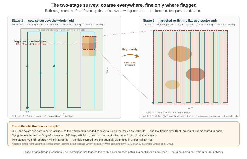
Two connections make this more than an agricultural aside. First, both stages are literally the Path Planning chapter’s lawnmower() — a bounding box, a spacing, an altitude — called twice: once with the field polygon and the coarse spacing, once with the flagged sector’s bounding box and the fine spacing. The generator was twenty lines precisely so that it could be re-parameterized like this. Second, the flag-then-re-fly structure is the running example’s own detect-then-investigate pattern wearing different clothes: the Path Planning chapter’s search grid is preempted by a detection and the aircraft goes to look, exactly as the coarse survey’s anomaly summons the targeted stage — except that here the “detection” is a depressed patch in a continuous index map rather than a bounding box from a neural network, a distinction the next section makes precise.
The research frontier collapses the two flights into one. A reinforcement-learning scouting agent that alternates in real time between an exploration phase — covering large swaths in search of regions that contradict its current map — and denser re-scouting over flagged problem regions, steered by a learned whole-field state estimate, reached 89.8 % field-assessment accuracy while sampling only 40 % of an 80-acre field, with the authors reporting 4.8× lower labor cost than exhaustive scouting; the whole-field state mattered, since an agent reasoning only from recently visited zones managed 80.3 % at the same coverage (Zhang et al. 2020). That is the two-stage doctrine made adaptive and continuous — and it is recognizably a cousin of the coverage-versus-investigate hinge this book built into the running example’s mission logic.
27.8 Two Paradigms, One Camera Mount
The chapter’s last obligation is precision about the contrast it has been trading on. Part III’s Building a Detection Pipeline chapter and this chapter both fly a camera over the ground and both end in a georeferenced claim about what is down there. Beneath that resemblance, they are solving different information-processing problems, and an engineer choosing between them should be able to name the differences exactly.
| Part III: RGB object detection | This chapter: multispectral index mapping | |
|---|---|---|
| Unit of inference | One frame at a time, onboard, at frame rate | One pixel at a time, across a whole orthomosaic |
| The computation | A learned function — millions of trained weights — mapping pixels to boxes and classes | A fixed arithmetic formula — a handful of band ratios — mapping reflectances to a physical index |
| What “detection” means | A discrete decision: this box is a goose with confidence 0.87, above threshold | A spatial anomaly: this patch’s continuous index sits below its surroundings |
| Output artifact | Bounding boxes and classes per frame, streamed live | A continuous scalar field over the field, assembled after landing |
| Ground truth required | A labeled dataset — thousands of hand-drawn boxes, the pipeline’s true bottleneck | Radiometric calibration — a panel, an irradiance sensor, a flight window |
| Fails when | The dataset lacked this case: unseen scale, lighting, or confusable species | Calibration breaks: cloud shadow, haze, sun angle, a skipped panel shot |
| Where it runs | The companion computer, subject to Part III’s latency and memory budgets | A workstation, deadline-free — photogrammetry is the cloud tier’s kind of work |
| Answers | “Is there a thing here, and what kind?” | “What is the condition of every point here?” |
The deepest row is the ground-truth one, because it names what each paradigm’s accuracy is made of. The detector’s competence is borrowed from its dataset: it knows what a goose looks like because thousands of examples said so, and it fails on what the dataset failed to contain. The index’s competence is borrowed from physics: nobody labeled examples of “stressed”; chlorophyll absorbs red, leaf structure scatters NIR, and the formula is the mechanism written as arithmetic. That is why the index generalizes to a field it has never seen with no retraining — and why it cannot, by itself, say goose: there is no per-pixel physical formula for a species. Each paradigm is the wrong tool for the other’s question.
The boundary, though, is a place to build, and the strongest recent results live on it. The machine-learning classifiers of both case studies above are learned functions on top of physically calibrated indices — the physics supplies invariant features, the learning supplies the disease-specific decision boundary. A very recent vineyard study went further and composed the paradigms outright: a YOLO object detector — the same family the running example’s Detector node runs — trained not on RGB frames but on imagery augmented with a chlorophyll-absorption index, locating Botrytis infection sites as discrete detections at 91.1 % F1, where the identical architecture on RGB alone managed 68.1 % (Montalban-Faet et al. 2026). Read against Table 27.1, that is the whole chapter in one experiment: the learned pipeline supplied the “find the discrete thing” machinery, and the physical index supplied 23 points of F1 that no amount of RGB data was going to.
The index-stack-plus-learning recipe generalizes past classification: one wheat leaf-rust study fed an algorithmically selected subset of UAV-derived vegetation indices into a neural network to predict continuous disease severity (\(R^2 \approx 0.78\) on validation), turning the healthy/diseased binary into a regression (Ju et al. 2023). On the flight-doctrine side, the incremental replanning machinery the Path Planning on the Edge chapter’s For More note introduced (D* Lite and kin) is what a single-flight adaptive scout needs when the “flagged sector” list changes mid-mission; the reinforcement-learning scouting paper is the current reference point for how far that can be pushed (Zhang et al. 2020). And for sensor selection — five-band versus dual-red-edge versus hyperspectral, fixed-wing versus multirotor per stage — the university extension literature is the practical, vendor-neutral starting point (North Carolina State University Extension 2021).
27.9 Check Your Understanding
- A field’s NDVI map shows a sharply depressed patch. The farm manager asks: “drought or disease?” Explain, in terms of what NDVI computes and what fungal infection does to the reflectance spectrum, why NDVI alone cannot answer — and what additional band measurements would begin to.
NDVI compresses the spectrum to one scalar per pixel from exactly two samples: red and NIR reflectance. Essentially every stressor — drought, nutrient shortage, fungal colonization, pest damage — erodes the same red/NIR contrast, so all of them converge to the same depressed index; the subtraction throws away the spectral shape that distinguishes the routes. The disease-discriminating information is concentrated in the red-edge region (~700–740 nm), which NDVI does not sample: fungal chlorophyll degradation and cell-structure collapse move and flatten the red-edge shoulder — and some diseases raise visible/red-edge reflectance while lowering NIR, an opposite-signed pattern distinct from drought’s flatter NIR-dominated depression. Measuring one or two red-edge bands (enabling NDRE, or REDSI with two of them) is the minimum addition that starts to separate the hypotheses; a targeted low-altitude re-fly or a scout’s visit confirms.
- Compute REDSI and NDRE for a pixel with \(\rho_R = 0.07\), \(\rho_{\text{RE1}}(705) = 0.13\), \(\rho_{\text{RE3}}(783) = 0.36\), and \(\rho_{\text{NIR}} = 0.41\) (take \(\rho_{\text{RE}} = \rho_{\text{RE1}}\) for NDRE). Then state which standard sensor class can compute each index and why.
REDSI \(= [40(0.36-0.07) - 118(0.13-0.07)]/(2 \times 0.07) = (11.6 - 7.08)/0.14 \approx 32\). NDRE \(= (0.41-0.13)/(0.41+0.13) = 0.28/0.54 \approx 0.52\). NDRE needs only NIR and one red-edge band, so any standard five-band agricultural array computes it. REDSI needs red plus two red-edge bands (≈705 and ≈783 nm); the standard five-band array carries only one red-edge filter, so REDSI requires a dual-red-edge multispectral rig (or hyperspectral, or the satellite bands it was validated on) — a concrete case of the index driving the sensor purchase.
- In the head-to-head validation, REDSI beat NDVI 84.1 % to 78.8 % at canopy scale and 85.2 % to 66.7 % at regional scale. A colleague concludes: “so a drone flying REDSI detects yellow rust at 85 % accuracy.” Name two distinct corrections that claim needs.
First, platform: the validation used Sentinel-2 satellite imagery at 10 m per pixel, not a drone. The index is sensor-agnostic and a UAV’s far finer GSD would plausibly do as well or better, but that was not tested — the published accuracy licenses a satellite claim, not a drone claim. Second, scope: 84–85 % is the accuracy for this disease (wheat yellow rust) with an index purpose-built for its red-edge signature, distinguishing it from background on those plots; it is not a general “disease detection accuracy,” and the same construction applied to a different pathogen or crop would need its own validation — as the stem-rust study’s different best-index set shows. (A third, finer point: quote accuracy per severity class where available; mild infection classifies worst and matters most.)
- The wheat stem-rust study reported per-class accuracies of 84 % (healthy), 76 % (mild), 97 % (moderate), 81 % (severe). Why is the pattern of those numbers — not the 85 % overall figure — the operationally decisive information for a grower deciding whether to buy the survey?
The economic value of the survey is concentrated in exactly one class: mild infection, the stage where fungicide intervention still preserves the crop. Moderate and severe infection are easy to classify (97 %, 81 %) precisely because the spectral perturbation is large — but by then a competent human scout sees it too, and much of the treatment window has closed. Mild is simultaneously the hardest class (76 %, the worst of the four) and the only one the flight is really for. The 85 % overall figure is an average dominated by classes that matter less; a grower should ask “how well does it catch what I can’t yet see?” — and the honest answer is the per-class number, roughly three in four. The general rule: early/low-severity detection performance, not headline accuracy, is the figure of merit for any early-warning sensing system.
- Using the chapter’s worked survey numbers (400 m × 400 m field; swath 51 m and spacing 15.4 m at 60 m altitude; both linear in altitude; 70 % side overlap throughout): compute legs, approximate track, and flight time for (a) one coarse pass at 8 m/s, and (b) a full-field pass at 20 m altitude and 5 m/s. Then (c) give the two-stage total if the coarse pass flags two sectors of 50 m × 50 m each, flown at 20 m and 5 m/s, and state the time ratio of (b) to (c).
- Given: 27 legs, ≈11.2 km, ≈23 min at 8 m/s. (b) At 20 m, swath and spacing scale by \(20/60\): swath 17 m, spacing ≈5.1 m; legs \(= \lceil 400/5.1 \rceil + 1 = 80\); track ≈ \(80 \times 400 + 79 \times 5.1 \approx 32.4\) km; at 5 m/s ≈ 6,480 s ≈ 108 min — plus several battery swaps. (c) Each 50 m sector at 5.1 m spacing: \(\lceil 50/5.1 \rceil + 1 = 11\) legs ≈ \(11 \times 50 + 10 \times 5.1 \approx 0.60\) km, ≈2 min at 5 m/s; two sectors ≈4 min plus transits. Two-stage total ≈ 23 + 4 ≈ 27 min against ≈108 min: a factor of ≈4 — and the two-stage plan still delivers the full fine-GSD imagery over the two sectors that actually matter, while fitting comfortably into a single battery cycle.
- A vendor brochure claims its drone service “detects Septoria leaf blotch seven days before visible symptoms at 97 % accuracy.” Based on this chapter, what should a careful engineer check before repeating that claim, and what is the actual provenance of those figures?
Check what was measured, on what platform, at what scale. The 7-day/97 % pairing traces to a study using a handheld proximal hyperspectral scanner imaging individual leaves — not a drone, not canopy scale, not aerial GSD. The underlying mechanism (spectral change preceding visible symptoms) genuinely motivates UAV red-edge sensing, but lead time and accuracy both degrade moving from a leaf millimetres from a scanner to a canopy tens of metres below a five-band camera — the late-blight work, for instance, went from 3-days-post-inoculation performance at leaf level to 5 at canopy level. Drone-platform lead times documented in this chapter run from roughly matching first visible symptoms, through a measured four-day lead at field scale, to weeks-early detection at reduced accuracy — a disease- and platform-specific range, not a transferable headline number.
27.10 Try It
Part 1 — build both indices and compare their anomaly maps. Simulate a calibrated five-band orthomosaic as five NumPy arrays (say 400 × 400, one metre per pixel) of reflectance values: start every band from a healthy baseline (visible bands low, red ≈ 0.05, red-edge ≈ 0.15, NIR ≈ 0.48, plus a few percent of spatial noise). Inject two anomalies with different signatures: a fungal patch (raise red and red-edge reflectance, lower NIR — the downy-mildew-style opposite-signed pattern) and a broad drought gradient (depress NIR and, mildly and proportionally, red-edge, leaving the visible shape mostly intact). Compute NDVI (Part I’s formula) and NDRE per pixel, render both as images with a shared color scale, and difference each against its healthy-area median to make anomaly maps. Write down what you see before rationalizing it: both indices should flag both anomalies, but compare the contrast each index draws between the two anomaly types — then compute a third map, the NDVI-to-NDRE ratio or difference, and check whether it separates the fungal patch from the drought gradient better than either index alone. Close with three sentences on what a single-index deliverable would have told the farm manager, and what the pair tells them.
Part 2 — plan the two-stage survey with the machinery you already own. Take your Part 1 anomaly map and threshold it (a percentile cut is fine; the ambitious version implements Jenks natural breaks) to flag anomalous pixels, then compute the flagged region’s bounding box. Now reuse the Path Planning on the Edge chapter’s lawnmower() exactly as written: call it once over the full field with the coarse-stage parameters from this chapter’s worked example (compute the spacing from a 51 m swath at 70 % overlap), and once over the flagged bounding box with the targeted-stage parameters (12.8 m swath, same overlap rule). Plot both paths over the anomaly map — coarse in one color, targeted in another — and audit the plan the way that chapter audited everything: total track length and flight time per stage, batteries required at your platform’s endurance, and the time you would have spent flying the whole field at targeted resolution instead. If you flew the running example’s missions in earlier chapters, note how little new code this took: the sensing payload changed everything about the pixels and nothing about the planner.
Related Lab: No lab currently maps to this chapter.
The running example will go back to chasing geese in a moment, but it is worth naming what this chapter demonstrated about the system the book has built: the coverage generator, the GSD arithmetic, the detect-then-investigate mission structure, and the discipline of asking what was actually measured all transferred to a sensing problem the running example never posed — which is what it means for engineering machinery to be general. What did not transfer is the part this Part is circling: a crop scout’s drone answers to the farmer whose field it flies, but a system that autonomously pursues wild animals answers to parties who never signed the work order. The account the previous chapter said no telemetry stream records is still owed, and the next chapter renders it.