22 Target Tracking and Visual Servoing
The previous chapter built the arbiter and left one box running on credit. HARASS_TARGET earned its full citizenship in the five-state machine — an entry guard with \(k\)-frame persistence, a dwell-time exit, stash-and-resume semantics under preemption — while its actual flying stayed deliberately thin: the Try It stubbed it as a fixed-radius orbit about the reported target, and the deterrence patterns themselves arrive in the next chapter. But between the arbiter and the patterns sits a premise that neither supplies. Every tick that HARASS_TARGET runs, it consumes a target track, and everything downstream — the dwell guard, the orbit stub, the swooping and circling patterns to come — assumes that track stays fresh for tens of seconds while the aircraft maneuvers aggressively around the very animal it is tracking. Nothing built so far makes that true. A track is fed by detections; detections come from a camera with a finite field of view; and the aircraft’s own motion is constantly working to carry the goose out of that field of view.
The Coordinate Frames chapter is why this gap carries a price tag rather than a vague unease. That chapter turned a bounding box and a depth value into a world-frame NED position — and then priced the result honestly: calibration, attitude error, synchronization, and depth uncertainty stack to perhaps half a metre at 6 m range, which is why it closed by insisting the transformed position be treated as an estimate to be refined — re-detected, re-transformed, and filtered as the aircraft approaches. Refinement has a precondition the transform cannot enforce: the goose must still be in the frame when the next image arrives. Fly toward a half-metre-wrong estimate of a moving bird, with a camera whose 640 columns span 90°, and a few seconds of accumulated error, target motion, and attitude transients will walk the bounding box to the image border and off it — at which point the detector goes silent, the track goes stale, and the position estimate that navigation depends on stops updating precisely when it is needed most. The machinery that prevents this is visual servoing: closing a control loop directly on what the camera sees, so that “keep the target in view” is not a hope but a feedback law. This chapter builds that law — a proportional controller whose error signal is measured in pixels — and makes the architectural argument the running example depends on: the image-plane loop and the world-frame estimate are not two answers to one question but answers to two different questions, and the system needs both.
22.1 Learning Objectives
- Distinguish position-based visual servoing (PBVS) from image-based visual servoing (IBVS) — what kind of sensor each treats the camera as, which space its error signal lives in, and which failure modes each inherits — and classify the running example’s existing detection-to-waypoint pipeline within that taxonomy.
- Derive the decoupled proportional centering law from first principles: pixel error from the image centre, normalization that makes the gains resolution-independent, the sign discipline that keeps the loop negative-feedback in PX4’s FRD/NED conventions, and deadband and saturation as the practical guards around it.
- Predict the closed-loop behavior of the centering loop quantitatively — its exponential time constant from the gain, the steady-state lag it leaves against a moving target, and the gain ceiling imposed by perception latency — using the same machinery as the Closed-Loop Control chapter, with pixel error as a new kind of error signal.
- Explain, at an introductory level, what the interaction matrix (image Jacobian) is, and why rotational centering channels are depth-independent while translational channels have loop gain that scales inversely with target range.
- Argue the “complementary, not redundant” two-loop architecture: an outer position-based loop that navigates on the Coordinate Frames chapter’s world-frame estimate, an inner image-based loop that keeps the target centered at frame rate — and why the inner loop is what keeps the outer loop’s estimate alive.
22.2 Key Vocabulary
- Visual servoing — controlling a robot’s motion by closing a feedback loop directly on live camera measurements, as opposed to look-then-move, in which vision is consulted once to plan a motion that then executes open-loop.
- Position-based visual servoing (PBVS) — the scheme that treats the camera as a 3D sensor: image measurements are first converted into a Cartesian position or pose estimate of the target, and the control error is computed in that 3D task space — “fly to where the goose is.”
- Image-based visual servoing (IBVS) — the scheme that treats the camera as a 2D sensor: the control error is computed directly in the image plane, as the offset between where a feature is and where it should be, with no 3D reconstruction inside the loop — “put the goose back in the middle of the picture.”
- Pixel error (centering error) — the image-plane offset \((e_x, e_y)\) between a detected feature’s pixel coordinates and its desired location, here the image centre; the error signal of the centering loop, and the only measurement it needs.
- Interaction matrix (image Jacobian) — the matrix \(\mathbf{L}\) relating the velocity of image features to the camera’s velocity, \(\dot{\mathbf{s}} = \mathbf{L}\,\mathbf{v}_c\); its entries depend on the target’s depth, which is why translational visual-servo channels need at least a rough range estimate to scale their gains.
- Deadband — a small zone around zero error inside which the controller commands nothing, so that a target already near-centered does not keep the aircraft hunting against detector noise.
- Gain scheduling — adjusting a controller gain as an operating condition changes; here, scaling the translational centering gain with the depth estimate so the loop behaves the same at 3 m as at 12 m.
- Target-following control loop — the complete cycle detection → pixel error → velocity/yaw-rate command → aircraft motion → new detection; a closed loop whose total latency sets how hard its gains can be pushed.
22.3 Two Ways to Use a Camera
The field’s standard taxonomy, established in the two tutorial papers every treatment of this subject descends from (Hutchinson, Hager, and Corke 1996; Chaumette and Hutchinson 2006), splits visual servo control by a single question: in which space does the error live?
Position-based visual servoing treats the camera as a 3D sensor. Image measurements — feature points, marker corners, a bounding box plus a depth value — are first pushed through a calibrated camera model into an estimate of the target’s position or pose in Cartesian space, and the controller drives a 3D error: the vector from where the vehicle is to where the estimate says it should be. The reader has already built one. The pipeline of the Coordinate Frames chapter — pixel and depth, through the intrinsics, through the fixed extrinsic rotation, through the attitude quaternion, out to a NED coordinate handed to navigation — is PBVS in everything but name. Its virtues are exactly the ones that chapter cashed in: the output is a geometrically meaningful world position, directly usable for waypoint navigation, standoff-distance logic, geofence checks, and logging where the goose was on a map. Its weakness was priced in the same chapter’s error budget: every link in the reconstruction — intrinsics, extrinsics, attitude, synchronization, depth — feeds its error straight into the commanded destination, with nothing inside the loop to notice or correct. And one more weakness went unstated there because no chapter yet needed it: nothing in a PBVS loop knows about the image border. The controller reasons entirely in world coordinates; it will happily command a maneuver that is correct in 3D and sweeps the target out of the camera’s field of view on the way.
Image-based visual servoing treats the camera as a 2D sensor and refuses the reconstruction step entirely. The error is computed where the measurement lives — in the image — as the offset between the feature’s current pixel coordinates and its desired ones, and that offset maps through a control law directly to motion commands. No pose estimate exists inside the loop, so no pose-estimation error can bias it: if the camera’s focal length is 5% wrong, or the mounting pitch is 2° off, an IBVS loop’s path to the goal bends, but its destination does not move, because the loop keeps pushing until the thing it actually measures — pixel error — reaches zero. The general IBVS control law, given in both tutorials, is a proportional law:
\[ \mathbf{v}_c = -\lambda\, \mathbf{L}^{+}\, \mathbf{e}, \]
where \(\mathbf{e}\) is the stacked image-feature error, \(\mathbf{L}^{+}\) is the pseudoinverse of the interaction matrix, and \(\lambda > 0\) is the gain. The interaction matrix is where IBVS keeps its one debt to 3D geometry: \(\mathbf{L}\)’s entries depend on the target’s depth \(Z\), so even a scheme that never reconstructs a pose needs a rough range to scale its commands sensibly — a point the next section makes concrete. IBVS’s classical pathologies are the mirror image of its virtues: it is only locally stable in general, and for large errors — especially large rotations — the commanded 3D trajectory can be strange, including the well-known camera retreat, where the camera backs away unnecessarily while sorting out a rotation (Chaumette and Hutchinson 2006).
| PBVS | IBVS | |
|---|---|---|
| Camera treated as | 3D sensor | 2D sensor |
| Error computed in | Cartesian/task space | the image plane |
| Needs in the loop | intrinsics, extrinsics, depth, attitude | pixel coordinates (plus rough depth for gain scaling) |
| Calibration error becomes | bias in the destination | distortion of the path |
| Keeps target in frame | no mechanism | that is the objective |
| Trajectory in 3D | clean, predictable, plannable | can be indirect or non-intuitive |
| Natural tasks | navigate to, stand off from, log a 3D position | center, point at, follow in view |
Two cautions before the table hardens into dogma. First, the “IBVS is robust, PBVS is fragile” summary is a statement about error structure, not a guaranteed performance ranking: in a direct head-to-head on a real robotic assembly task, a well-calibrated PBVS system converged faster and slightly more accurately than its IBVS counterpart, because once calibration is trustworthy, PBVS’s clean Cartesian trajectory wins and IBVS’s theoretical robustness edge has little left to pay for (Peng and Radke 2020). The trade-offs are real; their sign, in any given system, is an empirical question. Second, the schemes are endpoints of a spectrum, not a binary: hybrid formulations that blend a partial 3D estimate with image-plane features in one control law exist precisely because each pure scheme has failure modes the other lacks (Chaumette and Hutchinson 2006) — a fact the two-loop architecture later in this chapter exploits at the systems level rather than the control-law level.
For the specific task in front of the running example — keep a detected goose centered in the frame while the aircraft works around it — the choice is not close. “Target at image centre” is an image-space objective; reconstructing a 3D pose to answer “is the goose left or right of centre, and by how much” would launder a two-subtraction question through the entire error budget of the frame chain and hand back a worse answer, later. Applied UAV target-following systems make the same call, defining the error as the pixel offset between the detected feature and the desired (centered) position (Chen et al. 2021) and, in the simplest implementations, driving it with proportional or PID control. PBVS keeps the jobs it is actually good at — approach, standoff, mapping — and IBVS takes the one it was born for.
22.4 The Centering Law
The construction needs three ingredients: an error, a sign discipline, and two guards. All three fit in Figure 22.1.
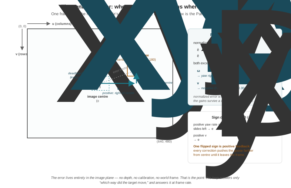
The error. Let the image be \(W \times H\) pixels with the origin at the top-left — the convention the Images as Data chapter fixed, \(u\) increasing rightward, \(v\) increasing downward — so the centre sits at \((c_x, c_y) = (W/2,\, H/2)\). The Part III detector reports a bounding box; its centroid \((u, v)\) is the feature. The pixel error is the componentwise offset,
\[ \begin{aligned} e_x &= u - c_x \qquad \text{(positive: target right of centre)} \\ e_y &= v - c_y \qquad \text{(positive: target below centre),} \end{aligned} \]
and dividing each component by its half-frame dimension normalizes it into \([-1, 1]\):
\[ \begin{aligned} \hat{e}_x &= \frac{e_x}{W/2} \\ \hat{e}_y &= \frac{e_y}{H/2}. \end{aligned} \]
The normalization looks cosmetic and is not. It makes the gains resolution-independent: a target one-quarter of the way to the frame edge produces \(\hat{e}_x = 0.5\) whether the camera is running its 640 × 480 depth-aligned mode or a 1280 × 720 mode, so a tuning session survives a camera-mode change, and the gains acquire honest physical units — radians per second of yaw, metres per second of climb, at full-scale error.
The law. The full IBVS machinery would build the interaction matrix for the centroid feature and invert it. For this task, the matrix collapses. One feature, near the image centre, at a roughly known working distance, controlled through two nearly decoupled channels — horizontal error corrected by yaw, vertical error corrected by vertical velocity — makes \(\mathbf{L}\) effectively constant and near-diagonal, so its pseudoinverse folds into two per-axis constants, and the general law \(\mathbf{v}_c = -\lambda \mathbf{L}^{+}\mathbf{e}\) specializes to two independent proportional controllers:
\[ \begin{aligned} \omega_z &= K_{\text{yaw}}\, \hat{e}_x \\ v_D &= K_{\text{alt}}\, \hat{e}_y, \end{aligned} \]
with \(\omega_z\) the commanded yaw rate, \(v_D\) the commanded vertical velocity in NED (positive down), and \(K_{\text{yaw}}, K_{\text{alt}} > 0\). This decoupled-proportional pattern is exactly the simplified form applied UAV tracking systems fly before the controller is upgraded (below); the justification for the simplification is the near-constancy of \(\mathbf{L}\) for this one-feature, small-error, known-ranges regime — push outside that regime (large errors, features far off-axis, unknown depth) and the full matrix earns its keep.
The signs. The alert reader will notice the minus sign of \(-\lambda \mathbf{L}^{+}\mathbf{e}\) has vanished, and the explanation is worth a paragraph because a wrong sign here is the single most common visual-servoing bug. What the general law’s minus sign encodes is negative feedback — commands must shrink the error — and whether that surfaces as a plus or minus in code depends entirely on the axis conventions at both ends of the loop. Trace the horizontal channel in the book’s conventions. In PX4’s FRD body frame, positive yaw rate swings the nose right. A camera panning right drags the whole scene left across the image: for a target near the centre, \(\dot{u} \approx -f_x\, \omega_z\), with \(f_x\) the focal length in pixels playing its geometric role as pixels per radian. So a target right of centre (\(\hat{e}_x > 0\)) commanded through \(\omega_z = K_{\text{yaw}}\hat{e}_x > 0\) yaws the nose right, slides the image left, and shrinks the error — two sign conventions (image-\(u\) rightward, FRD-yaw rightward) composing into a positive gain. The vertical channel composes the same way: positive \(\hat{e}_y\) (target below centre) commands positive \(v_D\) (descend, in down-positive NED), the descending camera slides the image up, and \(e_y\) shrinks. In a z-up convention — common in the literature — the same physics surfaces with minus signs, which is why published control laws disagree about signs while agreeing about everything real. The invariant to verify is never the symbol; it is the loop: does each channel’s command move the target toward the centre? Get one sign backwards and the loop is positive feedback — every correction pushes the goose farther out, exponentially, until it exits the frame in under a second. The Coordinate Frames chapter’s warning that a reflection in the transform surfaces in flight as mirrored behavior — steering left toward a target on the right — has a control-loop twin here, and the bench test in this chapter’s Try It exists to catch it before flight ever does.
The guards. Two practical amendments, both standard in fielded systems, complete the law. First, a deadband: inside a small normalized radius of the centre — 5% is typical, about 16 columns and 12 rows here — command zero. Detector centroids jitter by pixels frame to frame even on a stationary bird; without a deadband the loop dutifully chases that jitter, and the aircraft hunts — small perpetual yaw and climb oscillations that waste battery, smear the camera, and accomplish nothing, since a goose 15 pixels off-centre is exactly as tracked as one dead-centre. (One refinement worth knowing: commanding zero inside the band and \(K\hat{e}\) outside it puts a step discontinuity at the band’s edge, so implementations often subtract the band instead — command proportional to \(\hat{e}\) beyond the deadband — trading the step for a smooth ramp.) Second, saturation: clip each command to a ceiling well inside the airframe’s capability, for the same reason every state’s output in the previous chapter passed through the shared slew limiter — a bounding box appearing at the frame edge should produce a brisk turn, not a full-authority lunge that trades tracking accuracy for drama. The centering loop’s output joins every other behavior’s output at that same limiter; the loop decides direction and urgency, the limiter keeps the airframe’s experience continuous.
One structural fact about this law deserves to be stated before the numbers, because the whole architecture argument rests on it: the law says nothing about distance. Both channels rotate or translate the camera to re-point it; neither knows how far away the goose is, whether the aircraft is closing or retreating, or when to stop. A pure centering loop would keep a goose perfectly framed from 400 m away, forever. Approach and standoff belong to the world-frame estimate — which is the “complementary, not redundant” section’s business.
22.5 The Loop, Run by Numbers
Take the frame in Figure 22.1: the running example’s 640 × 480 camera, a confirmed track whose bounding-box centroid sits at \((u, v) = (480, 180)\) — upper right, a goose lifting away to the right of the aircraft’s nose. With gains \(K_{\text{yaw}} = 0.8\) rad/s and \(K_{\text{alt}} = 1.2\) m/s at full-scale error and a 0.05 deadband:
\[ \begin{aligned} \hat{e}_x &= \frac{480 - 320}{320} = +0.50 \\ \hat{e}_y &= \frac{180 - 240}{240} = -0.25, \end{aligned} \]
both far outside the deadband, so the loop acts:
\[ \begin{aligned} \omega_z &= 0.8 \times 0.50 = +0.40\ \text{rad/s} \approx 23^{\circ}/\text{s (yaw right)} \\ v_D &= 1.2 \times (-0.25) = -0.30\ \text{m/s (negative D: climb).} \end{aligned} \]
Yaw right at 23°/s, climb at 0.3 m/s — a firm, unhurried correction, reproducible on paper from four numbers and two gains.
What happens next is where the Closed-Loop Control chapter’s machinery takes over, because a pixel error is just an error signal, and this is just a P controller wearing a camera. Combine the image kinematics with the control law: \(\dot{e}_x = \dot{u} \approx -f_x \omega_z\) and \(\omega_z = K_{\text{yaw}} e_x / (W/2)\) give
\[ \dot{\hat{e}}_x = -\frac{f_x}{W/2}\, K_{\text{yaw}}\, \hat{e}_x, \]
a first-order exponential decay. The running example’s camera makes the constant memorable: a 90° horizontal field of view over 640 columns gave \(f_x = 320\) pixels in the Coordinate Frames chapter — exactly \(W/2\) — so the ratio is 1 and the normalized gain is the closed-loop bandwidth: time constant \(\tau = 1/K_{\text{yaw}} = 1.25\) s. From \(\hat{e}_x = 0.50\) the error decays to the 0.05 deadband in \(\tau \ln(0.50/0.05) \approx 2.9\) s, and the yaw rate decays with it — the proportional controller’s signature soft landing, no overshoot, no ringing, provided the gain respects the loop’s delay.
That proviso is the tuning story in one inequality. The error the controller acts on is old: roughly 50 ms of capture-to-publish pipeline (the Real-Time Inference chapter’s budget) plus up to one 20 Hz mission tick, call it a delay \(T_d \approx 0.1\) s. A proportional loop with pure delay, \(\dot{e}(t) = -K\,e(t - T_d)\), goes formally unstable when \(K\,T_d\) reaches \(\pi/2\) — here \(K \approx 15\) — but degrades long before: as \(K T_d\) grows past a few tenths, the controller is forever correcting an error that no longer exists, overshooting centre and swinging back, the same phase-lag mechanism the Closed-Loop Control chapter exposed. At \(K_{\text{yaw}} = 0.8\), \(K T_d = 0.08\) and the delay is invisible; crank the gain to 5 for “snappier” tracking and \(K T_d = 0.5\) buys visible hunting. The engineering rule is the usual one: the closed-loop time constant should sit an order of magnitude above the total loop delay, and the way to make the loop faster is to shrink the delay — a faster detector, a tick that reads fresher boxes — not to raise the gain into the oscillation regime.
Two more inherited results round out the analysis. A moving target turns the P controller’s steady-state error loose: a goose crossing the line of sight at 2.5 m/s at 10 m range subtends an angular rate of 0.25 rad/s, and holding the nose on it requires \(\omega_z = 0.25\) rad/s forever — which a proportional law only produces at a standing error \(\hat{e}_x = 0.25/0.8 \approx 0.31\), about 100 pixels. The goose rides a third of the way toward the frame edge, tracked but off-centre: the Closed-Loop Control chapter’s constant-disturbance standoff, re-materialized in pixels. The remedies are also that chapter’s — an integral term to grind the standing error away (with windup guards when the target accelerates), or feedforward of the track’s estimated angular rate — and the running example accepts the lag instead, because 100 pixels off-centre still leaves 220 pixels of margin, and simplicity is worth more here than perfection. Finally, depth: the yaw channel’s loop gain contains only \(f_x\) — rotation moves pixels at the same rate whatever the range, which is one reason yaw-based centering is the robust default. But the vertical channel is translational, and a translating camera moves a target’s image in proportion to \(f_y/Z\): the same 0.3 m/s climb that nudges a goose at 12 m nudges one at 3 m four times harder. A vertical gain tuned crisp at long range rings at short range. This is the interaction matrix’s depth-dependence stripped to one fraction, and the practical fix is one line of gain scheduling — scale \(K_{\text{alt}}\) with the depth estimate the outer loop already computes — or the conservative alternative, tuning at the closest working range and accepting sluggishness far out.
22.6 Complementary, Not Redundant
The system now holds two complete answers to “a goose was detected — do something”: the Coordinate Frames chapter’s transform, which produces a world position to navigate toward, and this chapter’s law, which produces re-pointing commands to keep the detection in frame. It is tempting to see them as rivals — the fast cheap loop versus the slow rigorous one — and to ask which the running example should use. The correct answer is that they are not answering the same question, and Figure 22.2 draws the architecture that uses both.
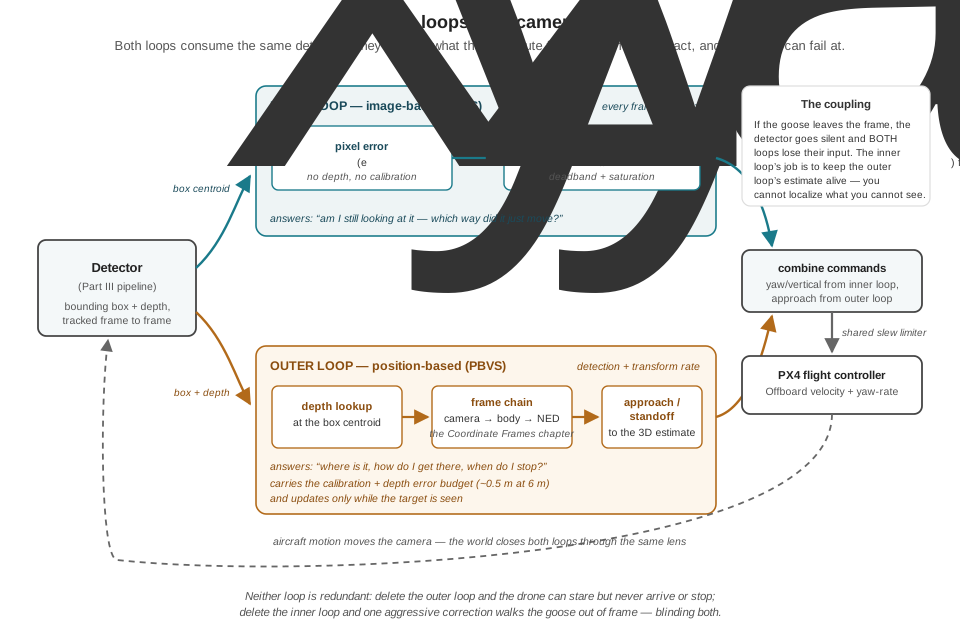
Run the failure analysis in both directions. A system with only the outer, position-based loop inherits the full error budget with no in-loop correction — the half-metre at 6 m is commanded, not just estimated — and, worse, nothing anywhere enforces that the target stays visible while the vehicle flies its correct-in-3D trajectory. One noisy depth sample, one aggressive correction, one goose that flaps ten metres during the estimate’s latency, and the bounding box crosses the image border. At that moment the failure compounds: the position estimate is built from detections, so losing sight doesn’t degrade the estimate, it stops it — the aircraft is now navigating to where a goose used to be, on a track aging toward the FSM’s 3 s dwell cutoff. You cannot localize what you cannot see. A system with only the inner, image-based loop fails in the complementary direction: it can hold the goose in frame from any distance, indefinitely, but it has no notion of range, closure, or standoff — it cannot approach, cannot stop approaching, cannot log where the goose is for the sweep planner, cannot answer a single question that the mission’s other consumers ask in world coordinates.
So the architecture stacks them, each at the rate its data supports. The outer loop runs at detection-plus-transform rate: box, depth, frame chain, filtered NED estimate, approach and standoff commands — the camera as 3D sensor, PBVS in spirit, feeding everything downstream that thinks in world coordinates. The inner loop runs every frame on raw pixel error — no depth lookup, no transform, nothing between the detector and the command but two subtractions and two multiplies — continuously absorbing exactly the errors the outer loop is blind to: target motion since the last estimate, attitude transients, the accumulated bias of calibration. The split is also an honest division by what can hurt each loop: the inner loop is immune to the calibration budget (it measures pixels and commands until pixels say centered) but knows nothing of the world; the outer loop knows the world but believes its calibration. Chained, the inner loop’s centering keeps the detection stream — the outer loop’s raw material — flowing, while the outer loop supplies the two things the inner loop structurally lacks: a range (which the vertical channel’s gain scheduling already wanted) and a destination.
This two-loop pattern is not an invention of convenience. At the control-theory level it is the systems-engineering cousin of hybrid visual servoing, which combines partial 3D estimates with image-plane features in one law precisely because the pure schemes fail differently (Chaumette and Hutchinson 2006). At the applied level it is how working UAV systems are built: a monocular precision-landing system for a moving platform, for instance, runs a fiducial-based localization stage to get the vehicle to the platform’s vicinity and image-plane PID corrections to keep the marker centered through the terminal approach (Salagame, Govindraj, and Omkar 2022) — coarse navigation from reconstruction, fine correction from pixels, the same architecture with a landing pad in place of a goose. And when the stakes or the dynamics outgrow proportional control, the error definition survives even as the controller is upgraded: a published UAV target-following system defines its objective as exactly this chapter’s centered-feature error and drives it with nonlinear model-predictive control (Chen et al. 2021) — the production-grade descendant of the same loop, solving for the command sequence rather than multiplying by a gain.
For the mission machine, the division of labor lands cleanly on the FSM’s states. SEARCH_GRID consumes the outer loop’s output at the moment of detection — the world-frame position that tells HARASS_TARGET where to go. HARASS_TARGET flies on both: the outer loop’s estimate governs approach and standoff radius, while the inner loop, ticking underneath, keeps the goose in frame so the track that entry guard confirmed stays fresh — feeding the dwell guard, feeding the estimate, and feeding the pattern generators the next chapter builds, every one of which (“swoop toward, circle around, feint away”) presumes the aircraft continuously knows which way the goose is. Harassment Pattern Generation will spend its pages on what to fly around a target; this chapter is why, throughout those maneuvers, there will still be a target to fly around.
22.7 The Centering Loop in Code
The law, its guards, and its conventions compress into one plain function, shaped — like everything the mission machine calls — to be invoked from the tick:
IMG_W, IMG_H = 640, 480   # the depth-aligned mode from Part III
DEADBAND = 0.05           # normalized: 5% of the half-frame
K_YAW = 0.8               # rad/s of yaw rate at full-scale error
K_ALT = 1.2               # m/s of vertical rate at full-scale error
MAX_YAW_RATE = 0.6        # rad/s   } ceilings well inside the airframe;
MAX_VERT_RATE = 0.8       # m/s     } the shared slew limiter still applies

def _p_channel(err, gain, limit):
    """One axis: deadband, then proportional, then saturation."""
    if abs(err) < DEADBAND:
        return 0.0                     # near-centered: don't hunt
    cmd = gain * err
    return max(-limit, min(limit, cmd))

def centering_command(bbox_center, image_size=(IMG_W, IMG_H)):
    """Pixel centroid of the tracked target -> (yaw_rate, vertical_rate).

    Signs follow PX4 conventions: positive yaw rate is nose-right (FRD),
    positive vertical rate is downward (NED). Both channels are negative
    feedback: each command moves the target's image toward the centre.
    """
    u, v = bbox_center
    w, h = image_size
    e_x = (u - w / 2) / (w / 2)        # [-1, 1], + = right of centre
    e_y = (v - h / 2) / (h / 2)        # [-1, 1], + = below centre
    yaw_rate = _p_channel(e_x, K_YAW, MAX_YAW_RATE)
    vert_rate = _p_channel(e_y, K_ALT, MAX_VERT_RATE)
    return yaw_rate, vert_rate
Wiring it into the previous chapter’s machine changes a handful of lines in the HARASS_TARGET case. The state’s action asked fly_pattern() to close on the target and work it; the centering loop now supplies the aim underneath whatever pattern is flown:
case MissionState.HARASS_TARGET:
    if self.track_is_fresh():          # measured or briefly coasted box
        yaw_rate, vert_rate = centering_command(self.track.bbox_center)
        self.fly_pattern(yaw_rate, vert_rate)  # pattern: next chapter
    else:
        self.hold_pattern()            # no fresh pixels: freeze the aim
    if self.target_gone(dwell=3.0):
        self.transition(MissionState.SEARCH_GRID, "resume sweep")
Three disciplines from the previous chapters carry over unchanged and are worth naming, because each guards a real failure. Freshness first: centering_command must only ever see a measured box — or one the Part III tracker is coasting through a few missed frames — never a stale one; servoing on a track that has been silent for a second steers the aircraft by a fiction, and the honest response to missing pixels is to freeze the aim and let the dwell guard, not the servo, decide what happens next (dead data is worse than no data, exactly as the FSM chapter argued for guards). One writer: the loop computes commands, but only the tick issues them — the centering law is a pure function called from the state’s action, not a callback with opinions about self.state. One limiter: its output merges with the pattern generator’s and passes through the same shared slew limiter as every other behavior, so a bounding box that jumps (an ID switch, a second goose) produces a bounded swing of the nose, not a snap.
The full interaction matrix is worth meeting once, even though this chapter’s task never inverts it. For a single image point at normalized coordinates \((x, y)\) and depth \(Z\), the classic result is a 2 × 6 matrix mapping the camera’s full velocity screw — three translations, three rotations — to the feature’s image velocity; its translational columns all carry \(1/Z\) while its rotational columns carry none, which is the general form of this chapter’s observation that yaw centering is depth-free and vertical-velocity centering is not (Chaumette and Hutchinson 2006). Stacking the matrices of several features and pseudoinverting yields servo laws that control all six degrees of freedom from imagery alone — the machinery behind precision manipulation and marker-based docking — at the price of the singularity and local-minimum pathologies the tutorials catalogue. The mature open-source implementation of all of it, PBVS and IBVS and the hybrid schemes, is INRIA’s ViSP library, which ships ROS integration and is a sensible next stop for a reader who wants to fly more than two channels. On the estimation side, production trackers rarely feed raw centroids to the servo: a constant-velocity Kalman filter over the track smooths detector jitter and supplies the angular-rate feedforward that eliminates the moving-target lag computed in this chapter — the same filter-then-control layering the reader has now seen at every level of the stack.
22.8 Check Your Understanding
- Classify each within the IBVS/PBVS taxonomy, with one sentence of justification: (a) the running example’s detection → depth → frame chain → NED waypoint pipeline from the Coordinate Frames chapter; (b) this chapter’s centering loop; (c) a precision-landing system that estimates a known-size fiducial marker’s full 3D pose and flies to a fixed offset above it.
- PBVS: the camera is used as a 3D sensor — image measurements are reconstructed into a Cartesian target position, and the error driven to zero (vehicle-to-waypoint) lives in task space. (b) IBVS: the error is the pixel offset from image centre, computed and controlled entirely in the image plane with no pose reconstruction in the loop. (c) PBVS, and a well-chosen use of it: the marker’s known geometry and the trusted calibration make the 3D reconstruction reliable, and the objective — a fixed spatial offset from the pad — is inherently a Cartesian goal, exactly the regime where PBVS’s clean, predictable trajectory is the advantage (Peng and Radke 2020).
- A camera runs at 1280 × 720. The tracked centroid is at \((u, v) = (400, 500)\), the gains are \(K_{\text{yaw}} = 0.6\) rad/s and \(K_{\text{alt}} = 1.0\) m/s at full-scale error, and the deadband is 0.08. Compute both commands, state each one’s physical direction, and then show what the same physical scene would command if the camera were switched to 640 × 360.
Centre is \((640, 360)\). \(\hat{e}_x = (400 - 640)/640 = -0.375\); \(\hat{e}_y = (500 - 360)/360 = +0.389\). Both magnitudes exceed the 0.08 deadband. Yaw: \(\omega_z = 0.6 \times (-0.375) = -0.225\) rad/s — negative is nose-left in FRD, correct for a target left of centre. Vertical: \(v_D = 1.0 \times 0.389 = +0.39\) m/s — positive D is downward, a descent toward a target below centre. At 640 × 360 the same scene puts the centroid at \((200, 250)\): pixel errors halve to \((-120, +70)\), but the half-frame normalizers halve too, so \(\hat{e}_x = -0.375\) and \(\hat{e}_y = +0.389\) exactly as before — the commands are identical. That invariance is what the normalization buys: gains tuned in one camera mode survive a mode change.
- A teammate ports a published centering law verbatim —
yaw_rate = -K * e_x_norm— onto the running example’s PX4 stack. Predict the flight behavior on the first confirmed detection, explain the mechanism in feedback terms, and describe a ground test that would have caught it.
The published law was almost certainly written for a z-up yaw convention; under PX4’s FRD (positive yaw = nose right) the minus sign turns the loop into positive feedback. A goose detected right of centre commands nose-left, the image slides right, the error grows, and the command grows with it: the error compounds exponentially and the goose exits the frame edge within a second or two, every correction accelerating the departure. The FSM survives — track lost, dwell expires, resume sweep — but harassment becomes structurally impossible, and the log shows the same signature every time: detection, brief yaw away, track lost. The catch-it-first test needs no flight: on the bench (or in SITL with a planted target), present a detection right of centre and assert the sign of the commanded yaw rate is positive — “target right must command nose right.” One assertion per channel, run against synthetic boxes at all four frame edges, pins all the sign conventions at once.
- The perception pipeline delivers boxes with 50 ms of end-to-end latency and the mission tick runs at 20 Hz, so the centering loop acts on errors up to about \(T_d = 0.1\) s old. For \(K_{\text{yaw}} = 0.8\) and for an impatient retune to \(K_{\text{yaw}} = 6\), evaluate \(K T_d\), describe the qualitative closed-loop behavior in each case, and state where the formal stability boundary lies. Which chapter’s machinery is this?
At \(K = 0.8\): \(K T_d = 0.08\), a factor of twenty below the instability boundary \(K T_d = \pi/2 \approx 1.57\) (i.e. \(K \approx 15.7\) for this delay); the closed-loop time constant \(\tau = 1/K = 1.25\) s dwarfs the delay, and the response is a clean exponential settle. At \(K = 6\): \(K T_d = 0.6\) — still formally stable but badly damped: the controller keeps acting on 100 ms-old error, repeatedly overshooting centre and swinging back, visible as the aircraft hunting left-right across the target. This is the Closed-Loop Control chapter’s phase-lag story with a new error signal: delay in the loop converts gain into oscillation, and the honest route to a faster loop is shrinking the delay (faster detector, fresher reads), not raising the gain toward the boundary.
- During a harassment run a goose walks steadily across the line of sight at 2 m/s at 8 m range. With \(K_{\text{yaw}} = 0.8\), compute where in the frame the P-only loop holds the goose at steady state, explain why the offset cannot decay to zero, and name the two standard remedies and the cost of each.
Required tracking rate: \(\omega = v/r = 2/8 = 0.25\) rad/s. A proportional law produces that only at a standing normalized error \(\hat{e}_x = 0.25/0.8 = 0.3125\) — about \(0.3125 \times 320 = 100\) pixels right of centre on the 640-wide frame, a steady lead the aircraft never closes. It cannot decay because zero error would mean zero commanded yaw rate, and a nose that stops turning immediately falls behind a target that does not stop moving — the same structural standoff as the Closed-Loop Control chapter’s proportional controller against a constant disturbance. Remedies: an integral term, which winds up the extra yaw rate until the error truly zeros but must be guarded against windup when the target reverses or the command saturates; or feedforward of the track’s estimated angular rate (e.g., from a Kalman filter over the track), which removes the lag without integral dynamics but is only as good as the rate estimate it is fed.
- Explain why \(K_{\text{yaw}}\) can be tuned once and trusted from 3 m to 30 m, while a \(K_{\text{alt}}\) tuned for crisp response at 12 m may oscillate as the aircraft closes to 3 m. Connect the explanation to the structure of the interaction matrix, and give the one-line fix.
Yaw is a rotational channel: a rotation sweeps every pixel at \(f_x\) pixels per radian regardless of how far away the scene is, so the loop gain contains no depth and the tuning is range-invariant. Vertical velocity is a translational channel: a camera translating at \(v\) moves a target’s image at \(f_y\,v/Z\) pixels per second, so the loop gain scales as \(1/Z\) — closing from 12 m to 3 m multiplies it by four, shrinking the effective time constant fourfold and pushing a crisply tuned loop toward the hunting regime. This is the interaction matrix’s structure in miniature: its translational columns carry \(1/Z\), its rotational columns do not — the precise reason IBVS needs at least a rough depth estimate even though it never reconstructs a pose. The fix is one line of gain scheduling: scale \(K_{\text{alt}}\) proportionally with the outer loop’s depth estimate (or, conservatively, tune at the closest working range and accept sluggishness far out).
22.9 Try It
Part 1 — build the law and pin its signs. Implement centering_command() exactly as in this chapter, then test it before any aircraft is involved. First, unit tests: boxes planted at all four frame edges and at centre must produce the four correct command signs and one all-zeros result; a centroid just inside the deadband must command zero on that channel while the other still acts; commands at full-scale error must clip at the ceilings. Second — the test that catches convention bugs — generate the inputs with the Coordinate Frames chapter’s inverse chain: plant a synthetic goose at a known NED position, use ned_point_to_optical() plus the intrinsics to project it to a pixel, and assert end-to-end that a goose planted east of a north-facing drone commands positive (rightward) yaw. Then close the loop kinematically, no simulator yet: in a small script, hold the goose fixed in NED, integrate the commanded yaw rate and vertical rate into the drone’s pose at 20 Hz with a 0.1 s command delay, re-project the goose each step, and plot \(\hat{e}_x(t)\). Verify the exponential settle and measure its time constant against the predicted \(1/K_{\text{yaw}}\); then raise \(K_{\text{yaw}}\) until the trace hunts, and check the onset against the \(K T_d\) arithmetic.
Part 2 — wire it into the machine and track something that moves. In SITL, replace the previous chapter’s HARASS_TARGET stub aim with centering_command(), fed by a scripted target that the simulation projects into synthetic bounding boxes (the Part 1 projection code, now driven by a moving NED trajectory): a goose that holds still for 5 s, walks at 2 m/s across the line of sight for 10 s, then flaps away at 6 m/s. Log pixel error, commanded rates, and the FSM state at full rate. Confirm four behaviors against this chapter’s numbers: the initial centering settles with the predicted time constant; the walking phase holds the goose at the predicted steady-state offset (\(\hat{e} = \omega_{\text{target}}/K_{\text{yaw}}\) — compute it from your geometry before you fly it); the deadband keeps the aircraft quiet, not hunting, when the goose is stationary; and the flap-away phase either tracks or cleanly loses the target into the FSM’s dwell logic — kill the synthetic detections mid-run and confirm the aim freezes and the 3 s dwell, not the servo, hands control back to SEARCH_GRID with a [STATE CHANGE] line that explains itself. Finish with the sign-flip experiment from the checks: negate one gain, re-run the stationary phase, and keep the plot of the error diverging exponentially — the clearest picture of positive feedback a logbook can hold.
Related Lab: See Appendix B for the lab assignment that applies this chapter’s concepts.