19 Path Planning on the Edge: Search Grids and Coverage Algorithms
The Coordinate Frames chapter closed by handing this Part a stream of imperfect world-frame targets and asking what a planner does with them. Before that question can be answered, there is an older debt to pay. Back in Part II, the Mission Scripting chapter flew a lawnmower survey that had been clicked out by hand on QGroundControl’s map — and admitted, in the same breath, that the pattern was not an aesthetic choice but a computable one: the row pitch is a sensor parameter, and “the entire pattern can be computed from the field polygon and the sensor footprint.” This chapter performs that computation. It is the first planning algorithm of the book, and deliberately the simplest: a function that takes a bounding box and a sweep spacing and returns the ordered NED waypoint list the Mission Scripting chapter’s state machine already knows how to fly.
The chapter then does something the hand-drawn version never had to: it asks what the algorithm is for, and when it is the wrong tool. A lawnmower path answers one specific question — how does a drone with a finite sensor footprint guarantee it has seen every point of an area? — and it answers it without a map, without obstacles, and in microseconds of arithmetic. The other canonical planning question — how do I get from here to there, past things in the way? — belongs to a different family entirely: graph search, whose standard-bearer is A*. The running example needs both. Searching an open field for geese is a coverage problem; closing on a detected goose, re-routing when the world changes, and threading obstacles are point-to-point problems. Knowing which question is being asked, before reaching for an algorithm, is most of what “path planning” means in practice — and both algorithms here are chosen for the same reason the rest of the stack was: they run comfortably on the low-power companion computers of Part I, where planning shares a processor with inference and telemetry.
19.1 Learning Objectives
- Derive a sweep-line spacing from sensor geometry — altitude, field of view, and required overlap — and explain why the Mission Scripting chapter’s hand-drawn 6.5 m row pitch is the number this arithmetic produces.
- Implement the lawnmower (parallel-sweep) path generator: given a bounding box and a maximum spacing, compute the leg count, the exact spacing, and the ordered boustrophedon waypoint list.
- Define cross-track error, compute the per-leg error budget that keeps adjacent swaths overlapping, and explain why minimizing it is a coverage guarantee rather than a cosmetic preference.
- Describe A* search on an occupancy grid — the roles of \(g\), \(h\), and \(f = g + h\) — and state the admissibility condition under which it returns a shortest path.
- Decide, for a given mission phase, whether the planning question is area coverage or point-to-point navigation, and select and parameterize the appropriate algorithm — including when dynamic re-routing forces the choice to be revisited in flight.
19.2 Key Vocabulary
- Coverage algorithm — a path planner whose goal is not to reach a point but to pass a sensor’s footprint over every point of a region; its output is judged by completeness of coverage, not by path length to a destination.
- Lawnmower search pattern (parallel sweep, boustrophedon) — the canonical coverage path: long parallel legs spaced at most one sensor swath apart, joined by short row steps, flown in alternating directions so each leg begins where the last one ended.
- Search bounding box — the axis-aligned rectangle \([x_{\min}, x_{\max}] \times [y_{\min}, y_{\max}]\), expressed here in local NED coordinates, that defines the region a search must cover; together with the spacing, the complete parameterization of a lawnmower path.
- Swath width (\(w\)) — the width of ground a downward-looking sensor images along one leg, set by altitude and field of view; the physical quantity the sweep spacing must not exceed.
- Sweep spacing (\(s\)) — the perpendicular distance between adjacent legs; chosen as the swath width derated by a deliberate overlap fraction, so that imperfect flying still leaves no unseen strip.
- Cross-track error (\(e_{ct}\)) — the perpendicular distance from the vehicle’s actual position to the straight line of its current leg; the along-track coordinate measures progress, the cross-track coordinate measures straying.
- A* search — best-first graph search that expands nodes in order of \(f(n) = g(n) + h(n)\), the cost incurred so far plus a heuristic estimate of the cost remaining; with an admissible heuristic it returns a minimum-cost path.
- Admissible heuristic — a heuristic that never overestimates the true remaining cost (straight-line distance is the standard example for spatial planning); the property that upgrades A* from “usually good” to provably optimal.
- Dynamic re-routing — re-planning in flight when the world model changes — a new obstacle, a moved target, an updated cost map — either by re-running the planner or by incremental methods that repair the previous solution instead of discarding it.
19.3 The Spacing Comes from the Sensor
Every parameter of a lawnmower path except one is geometry the operator already owns: the bounding box is the field to be searched, the altitude is fixed by the mission (5.5 m for the running example’s survey, comfortably under the regulatory ceiling), and the leg length falls out of the box. The one genuinely new number is the sweep spacing, and it comes from the camera.
A camera looking straight down from altitude \(h\) with a horizontal field of view \(\theta_{\text{fov}}\) images a strip of ground — the swath — whose width is a single line of trigonometry: half the swath subtends half the field of view, so
\[ w = 2\,h \tan\!\left(\frac{\theta_{\text{fov}}}{2}\right). \]
The running example’s depth camera was estimated in the Coordinate Frames chapter to have roughly a 90° horizontal field of view. At the survey altitude:
\[ w = 2 \times 5.5 \times \tan 45^\circ = 11.0\ \text{m}. \]
Flying adjacent legs exactly 11 m apart would tile the field with zero margin: any imperfection — a metre of GNSS scatter, a gust, a goose at the seam between swaths imaged too obliquely to detect — opens an unseen strip. The standard remedy is to derate the spacing by an overlap fraction \(\beta\):
\[ s = w\,(1 - \beta), \]
and \(\beta = 0.4\) — a common choice when detection reliability at the swath edges is doubtful — gives \(s = 11.0 \times 0.6 = 6.6\) m. Here the book’s threads tie together pleasingly: the real hand-drawn survey that the Mission Scripting chapter dissected had a row pitch of roughly 6.5 m, drawn by eye on a map. The eye was right, and now it is clear why it was right: 6.5 m is what a 90° camera at 5.5 m altitude with 40 % overlap requires. The hand and the arithmetic agree — but only the arithmetic scales, transfers to a new altitude, and can run on board.
Two caveats keep the model honest. First, the formula assumes a nadir-pointing camera; the running example’s camera is pitched 45° forward (the extrinsic the Coordinate Frames chapter calibrated), which projects a trapezoidal footprint ahead of the aircraft rather than a rectangle below it. The conservative practice is to use the footprint’s narrowest cross-track extent as \(w\), and the nadir formula is a serviceable stand-in at survey altitudes. Second, the formula is the reason the search flies at constant altitude: \(w\) scales linearly with \(h\), so an altitude that wanders makes the swath width wander with it, and a spacing chosen for 5.5 m silently loses its overlap margin at 4 m. Constant altitude is not a stylistic requirement — it is what holds \(w\), and therefore the coverage guarantee, still.
19.4 The Generator: Two Parameters In, a Mission Out
With \(s\) in hand, generating the path is a short exercise in careful bookkeeping. The region is an axis-aligned bounding box in local NED — \([x_{\min}, x_{\max}]\) north–south, \([y_{\min}, y_{\max}]\) east–west — and the legs will run north–south (the long axis), stepping east between legs. Three decisions make the algorithm correct rather than merely plausible:
- Round the leg count up, never the spacing. The box width \(W = y_{\max} - y_{\min}\) is rarely an exact multiple of \(s\). Taking \(n = \lceil W / s_{\max} \rceil + 1\) legs and then recomputing the actual step as \(W / (n - 1)\) shrinks the spacing to fit — the step can only come out at or below the maximum the sensor allows, so rounding can tighten coverage but never loosen it.
- Alternate leg directions. Even-indexed legs fly south-to-north, odd-indexed legs north-to-south. Each leg then begins where the previous one ended, and the row step between legs needs no waypoint of its own — it is simply the flight from one leg’s last waypoint to the next leg’s first.
- Emit waypoints, not trajectories. The output is an ordered list of \((N, E, D)\) triples — exactly the data structure the Mission Scripting chapter’s NAVIGATE state consumes, streaming each waypoint as an Offboard setpoint and advancing on the acceptance-radius arrival test. The planner plans; the machinery that flies is already built.
import math

def lawnmower(x_min, x_max, y_min, y_max, s_max, altitude):
    """Parallel-sweep (lawnmower) coverage path over a NED bounding box.

    Legs run north-south (along x); the sweep steps east (along y).
    Returns an ordered list of (north, east, down) waypoints.
    """
    width = y_max - y_min
    n_legs = max(2, math.ceil(width / s_max) + 1)
    step = width / (n_legs - 1)      # actual spacing: <= s_max by construction
    z = -altitude                    # NED: down is positive, so up is negative
    waypoints = []
    for i in range(n_legs):
        y = y_min + i * step
        if i % 2 == 0:               # even legs: fly south -> north
            waypoints.append((x_min, y, z))
            waypoints.append((x_max, y, z))
        else:                        # odd legs: fly north -> south
            waypoints.append((x_max, y, z))
            waypoints.append((x_min, y, z))
    return waypoints
Twenty lines, no dependencies beyond ceil, and a run time measured in microseconds — a planner that could re-run every second on the smallest computer in Part I’s inventory without anyone noticing. Figure 19.1 traces a worked call: a fresh illustrative search area, a 60 m × 33 m box north-east of the launch point, at the survey’s 5.5 m altitude with \(s_{\max} = 6.6\) m.
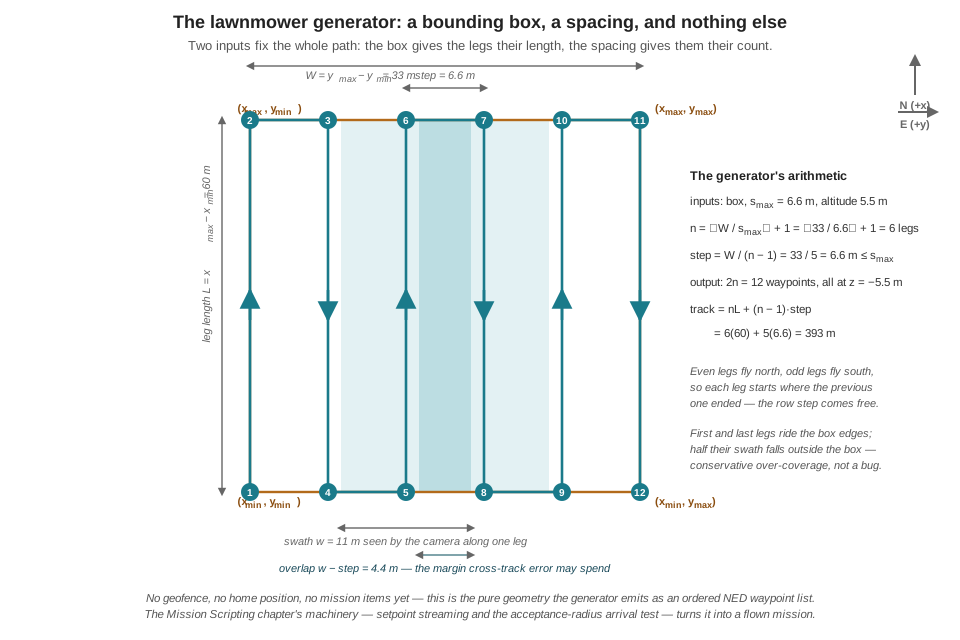
Follow the arithmetic through. \(W = 33\) m and \(s_{\max} = 6.6\) m give \(n = \lceil 5.0 \rceil + 1 = 6\) legs, and the recomputed step is \(33 / 5 = 6.6\) m exactly. Six legs of 60 m and five row steps of 6.6 m make the total track
\[ d = nL + (n-1)\,s = 6(60) + 5(6.6) = 393\ \text{m}, \]
and the track length immediately audits the schedule, the same trick the Mission Scripting chapter played on its plan file. At that survey’s camera-friendly 1.5 m/s:
\[ t = \frac{393}{1.5} = 262\ \text{s} \approx 4.4\ \text{min}, \]
which busts the 3.5-minute search-leg allocation in Part I’s mission time budget. At 2.0 m/s the same path takes 197 s ≈ 3.3 min and fits. This is the kind of trade a generator surfaces before anything flies: spacing is quantized (the \(\lceil\cdot\rceil\) means widening \(s_{\max}\) only drops a whole leg at discrete thresholds — here, not until \(s_{\max} \ge 8.25\) m, a 25 % overlap), while speed is continuous, so speed is usually the first lever pulled. Whether the detector still performs at 2.0 m/s of motion blur is a question for the frame-rate and latency budgets of Part III — planning decisions ripple into perception, and the budget arithmetic is where the ripple shows up.
The computed version also settles an audit the hand could not. The Mission Scripting chapter’s real survey put four legs at 6.5 m pitch — spanning about 19.5 m — inside a fenced field nearly 39 m across. Run the generator on that fence and it asks for seven legs, not four: the hand-drawn mission swept roughly half its field, a shortfall invisible on the map view and instant in the arithmetic. Nothing about the flight was wrong; the coverage claim was, and only the computation noticed.
Two practical notes complete the generator. Real search areas are rarely aligned with north: the standard treatment is to rotate the region’s corner coordinates into an axis-aligned frame, generate the path there, and rotate the waypoints back — a single 2D rotation matrix each way, machinery the Coordinate Frames chapter made routine. And the bounding box must sit strictly inside the geofence polygon of the Geofencing and Fail-Safes chapter, with margin for the cross-track error the next section budgets — a generated path that grazes the fence line is a generated failsafe trigger.
19.5 Cross-Track Error Is a Coverage Budget
The generator’s output is a guarantee written in pencil: if the aircraft flies each leg where the arithmetic put it, every point of the box passes under the camera. The quantity that measures “where the arithmetic put it” is cross-track error. For the leg from waypoint \(A\) to waypoint \(B\), define the unit tangent and normal
\[ \hat{t} = \frac{B - A}{\lVert B - A \rVert}, \qquad e_{ct} = (p - A) \cdot \hat{n}, \]
where \(p\) is the vehicle’s estimated position and \(\hat{n}\) is \(\hat{t}\) rotated 90° in the horizontal plane. The projection onto \(\hat{t}\) is the along-track coordinate — how far down the leg the vehicle has progressed; the projection onto \(\hat{n}\) is the cross-track coordinate — how far it has strayed off the line. A signed \(e_{ct}\) (positive right of track, negative left) is more useful than a distance, because its sign says which way to steer back.
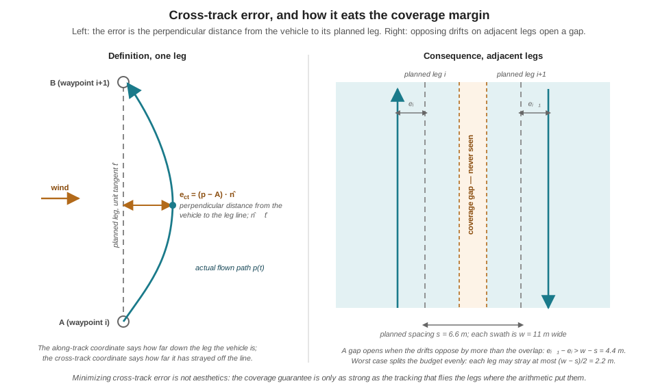
Figure 19.2 shows why this number owns a line in the mission requirements rather than a footnote. The swath of a leg flown with error \(e_i\) is displaced by \(e_i\); adjacent swaths, planned to overlap by \(w - s\), stop overlapping when the two legs drift apart by more than that margin:
\[ e_{i+1} - e_i > w - s \quad\Longrightarrow\quad \text{a strip between legs is never imaged.} \]
For the worked numbers, \(w - s = 11.0 - 6.6 = 4.4\) m, and the worst case — adjacent legs drifting in opposite directions — splits the budget evenly: each leg may stray at most \((w - s)/2 = 2.2\) m before the coverage claim fails. Now the budget can be spent, item by item, and the items are all familiar. The position estimate itself carries metre-scale GNSS scatter — the same scatter that set the floor under the Mission Scripting chapter’s acceptance radius — and the vehicle can only hold the line as well as it knows where the line is. Steady wind adds a systematic offset: the position controller flies crabbed into the wind, converging to the leg with some residual bias rather than tracking it exactly. And the acceptance radius contributes at the leg ends: with the 1.5 m radius that chapter chose, each corner is cut up to 1.5 m before the turn begins, shaving the swath short at the box’s north and south edges. Metre-scale error against a 2.2 m budget is not comfortable — it is roughly half the budget spent before the wind blows — which is precisely why the requirement is phrased minimize cross-track error, and why the overlap fraction \(\beta\) exists at all: \(\beta\) is the coverage guarantee’s insurance policy, priced in extra legs and minutes of battery.
One subtlety separates good leg-tracking from naive waypoint-chasing. A controller that simply steers at the next waypoint from wherever it currently is will happily fly a diagonal back to the corner after a gust — correct arrival, wrong swath, since the diagonal’s camera footprint is not the planned leg’s. Tracking the line — feeding the controller a setpoint that advances along the leg while nulling \(e_{ct}\) — keeps the flown swath congruent with the planned one. The cascaded position controller of Part II does this well when the streamed setpoints march down the leg at the commanded ground speed rather than jumping to the far corner in one step; the distinction costs a few lines in the NAVIGATE state and buys back most of the wind’s share of the budget.
19.6 A Different Question: A* and Point-to-Point Planning
The lawnmower generator never looked at a map, because its problem statement contains no obstacles: an open field, a box, a sensor. The moment the question changes from see everything to reach that point — fly to the detected goose behind the treeline, return home around the buildings, re-route when the fence’s safe corridor closes — coverage machinery has nothing to offer, and the problem becomes search on a graph.
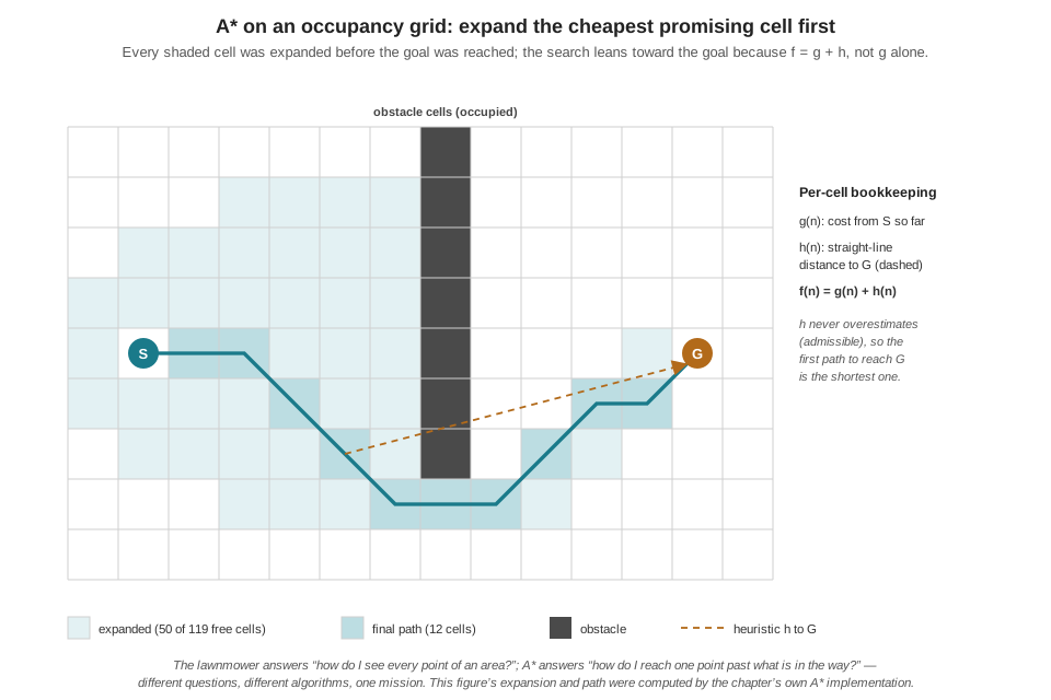
The standard discretization is an occupancy grid: the world chopped into cells, each marked free or occupied, with free cells connected to their neighbors (8-connectivity, with diagonal moves costing \(\sqrt{2}\) times a cell). A path is a walk through free cells from start to goal; the shortest such walk is the object of interest. Breadth-first search would find it by expanding uniformly in all directions; Dijkstra’s algorithm generalizes to weighted cells but shares the blindness. A* adds the one idea that makes graph search practical on small computers: expand next the node that looks cheapest overall, where “looks” combines the cost already paid with an optimistic estimate of the cost remaining,
\[ f(n) = g(n) + h(n), \]
with \(g(n)\) the accumulated cost from the start and \(h(n)\) the heuristic — for spatial planning, the straight-line (Euclidean) distance to the goal. The estimate is admissible: a straight line ignores every obstacle, so it can only under-estimate the true remaining cost, never over-estimate it. Admissibility is the load-bearing property — it guarantees that when the goal is first selected for expansion, no cheaper path to it remains undiscovered, so the path returned is optimal.
import math, heapq

def a_star(grid, start, goal):
    """Shortest path on an occupancy grid; returns a list of cells or None."""
    def h(c):
        return math.hypot(c[0] - goal[0], c[1] - goal[1])

    open_heap = [(h(start), start)]        # priority queue ordered by f
    g = {start: 0.0}
    parent = {}
    closed = set()
    while open_heap:
        _, current = heapq.heappop(open_heap)
        if current in closed:
            continue                       # stale queue entry; already done
        if current == goal:
            path = [goal]
            while path[-1] != start:
                path.append(parent[path[-1]])
            return path[::-1]
        closed.add(current)
        for nbr, step_cost in free_neighbors(grid, current):
            tentative = g[current] + step_cost
            if tentative < g.get(nbr, math.inf):
                g[nbr] = tentative
                parent[nbr] = current
                heapq.heappush(open_heap, (tentative + h(nbr), nbr))
    return None                            # goal unreachable
The structure to notice: a priority heap ordered by \(f\), a g table recording the best known cost to each cell, and relaxation — a neighbor is re-queued whenever a cheaper route to it appears. Figure 19.3 shows the algorithm’s signature behavior on a small grid with a wall between start and goal: the expansion does not flood outward uniformly (that would be Dijkstra) but leans toward the goal, spilling around the obstacle only as far as the heuristic’s optimism is contradicted by the wall.
What does this cost on a companion computer? Less than intuition suggests, at mission scales. A 100 m × 100 m working area at 0.5 m resolution is a 200 × 200 grid — 40,000 cells — and a full A* query over it completes in single-digit milliseconds in interpreted Python, far faster compiled; even a 3D grid with twenty altitude layers stays under a million nodes. The genuine constraints on the edge are different ones. Memory scales with the map, not the path, so resolution is chosen to fit the vehicle, not the cartographer’s ambition. And the rate of planning matters more than the cost of one plan: a world that changes — a goose that moves, an obstacle that appears in the depth camera — invalidates the current path and demands dynamic re-routing. The blunt approach, re-running A* from the vehicle’s current cell, is often affordable at these grid sizes and is the right first implementation. When it is not affordable — larger maps, faster replan rates — the practical toolkit is a family of A* variations: weighted A*, which multiplies the heuristic by \(\varepsilon > 1\) to expand far fewer nodes at the price of a path at most \(\varepsilon\) times optimal (a bargain when \(\varepsilon = 1.5\) halves the compute); and incremental planners in the D* Lite family, which repair the previous search when a handful of edge costs change instead of starting from nothing — the standard answer when re-routing runs inside a control loop.
19.7 Two Planners, One Mission
Set side by side, the two algorithms are less rivals than answers to different questions, and the running example’s mission asks both in sequence:
| Lawnmower coverage | A* graph search | |
|---|---|---|
| Question answered | “Have I seen every point of the area?” | “What is the shortest way to that point?” |
| World model required | None — a bounding box and a sensor footprint | An occupancy grid or graph with costs |
| Obstacles | Assumed absent (open field) | The entire point |
| Output | Fixed waypoint list, known length in advance | Path dependent on the map; length known only after search |
| Guarantee | Complete coverage, if cross-track error stays within the overlap margin | Minimum-cost path, if the heuristic is admissible |
| Compute cost | Microseconds, independent of world size | Milliseconds and up, scales with map size and clutter |
| Mission phase | Systematic search for a target | Transit, approach, and re-routing around obstructions |
The handoff between them is the mission’s hinge, and it is worth being precise about the mechanics. The lawnmower list is flown by the Mission Scripting chapter’s state machine — stream the current waypoint, advance on the acceptance test — inside a state the Finite State Machines and Behavior Trees chapter will name SEARCH_GRID. The search-phase requirement is that a detection immediately preempts the sweep: the machine abandons the current leg mid-flight and transitions to pursuit, exactly the event-driven preemption the state-machine formalism was built for. Two design consequences follow for the planner. First, because the path is data — a list and an index — abandoning it costs nothing and resuming it costs one integer: store the index, chase the goose, and re-enter the list at the stored leg when the pursuit resolves, rather than re-sweeping ground already covered. Second, the pursuit target arrives from the perception stack as a NED position — the very stream of imperfect world-frame targets the Coordinate Frames chapter delivered — and whether the pursuit needs A* at all depends on the world between drone and goose: over the open field, the answer is usually a straight line and no planner; near the treeline or a geofence boundary, it is a grid query. The next chapters take up what happens after arrival — the deterrence patterns flown at the target, and the state machinery that sequences search, pursuit, and escape into one mission.
The lawnmower over a rectangle is the base case of a richer theory. Boustrophedon cellular decomposition extends complete coverage to regions with obstacles: the free space is sliced into obstacle-free cells by sweeping a line across the region and splitting wherever an obstacle interrupts it; each cell gets its own lawnmower, and the cells are visited in an order that minimizes transit — a traveling-salesman flavored sequencing problem. Energy-aware variants choose leg orientation as well: legs aligned with the prevailing wind trade fewer turns against asymmetric headwind/tailwind legs, a measurable difference in battery on large fields. On the graph-search side, the D* Lite algorithm mentioned for re-routing maintains its search rooted at the goal, so that when the vehicle moves or costs change, most of the computed structure survives — the reason it became the standard for planetary rovers and remains the default answer when A* must run inside a tight replanning loop.
19.8 Check Your Understanding
- A drone searches at 8 m altitude with a nadir camera whose horizontal field of view is 90°, and the mission requires 30 % swath overlap. Compute the swath width and the sweep spacing, then the number of legs the generator emits for a bounding box 50 m wide.
Swath: \(w = 2 \times 8 \times \tan 45^\circ = 16\) m. Spacing: \(s = 16 \times (1 - 0.3) = 11.2\) m. Legs: \(n = \lceil 50 / 11.2 \rceil + 1 = \lceil 4.46 \rceil + 1 = 6\), and the recomputed step is \(50 / 5 = 10\) m — tighter than the 11.2 m maximum, as the ceiling guarantees. The generator never widens the spacing to fit the box; it adds a leg and shrinks the step.
- Trace
lawnmower(0, 100, 0, 20, 7.0, 6.0)by hand: how many legs and waypoints result, what is the actual step, in which direction does the third leg (index 2) fly, and what is the final waypoint?
\(W = 20\), so \(n = \lceil 20/7 \rceil + 1 = 3 + 1 = 4\) legs and \(8\) waypoints, with step \(20/3 \approx 6.67\) m. Leg index 2 is even, so it flies south-to-north (\(x\) from 0 to 100) at \(y \approx 13.33\) m. The last leg (index 3, odd) flies north-to-south at \(y = 20\), so the final waypoint is \((0, 20, -6.0)\) — northing 0, easting 20 m, 6 m above the launch altitude in NED’s negative-down convention.
- A survey flies \(w = 11\) m swaths at \(s = 8\) m spacing. GNSS scatter alone contributes about 1 m of cross-track error per leg. How much additional systematic drift (wind bias) per leg can the coverage guarantee absorb in the worst case, and what are the two remedies when the answer is judged too thin?
The overlap margin is \(w - s = 3\) m, and the worst case is adjacent legs drifting oppositely, so each leg’s total budget is \((w-s)/2 = 1.5\) m. With 1 m already spent on GNSS scatter, only about 0.5 m per leg remains for systematic wind bias — thin, since steady crosswind residuals can exceed that. The remedies pull opposite levers: tighten the spacing (more overlap, more legs, more time and battery) or reduce the error itself (track the leg line rather than chase corners, feed the controller setpoints that march along the leg, accept the time cost of flying slower in wind).
- A* with the Euclidean heuristic returns an optimal path. A colleague proposes doubling the heuristic — using \(h'(n) = 2\,h(n)\) — because it makes the planner visibly faster on the companion computer. What property is lost, what is the worst case for the returned path, and why might the trade still be accepted on a drone?
Doubling breaks admissibility: \(h'\) can now overestimate the true remaining cost, so the goal can be expanded while a cheaper route is still unexplored, and optimality is lost. This is weighted A* with \(\varepsilon = 2\); the returned path is at most \(2\times\) the optimal cost (bounded suboptimality), and in open maps typically far closer. The trade is often right on a drone because the planner shares a small processor with inference and telemetry, and a path 10–20 % long that arrives in a fifth of the compute — and therefore replans at a higher rate as the world changes — beats a perfect path delivered late.
- For each task, name the appropriate planner — lawnmower coverage, A*, or neither — and justify in one sentence: (a) sweep a 70 m × 40 m open field to find any geese present; (b) fly from the field’s corner to a detected goose on the far side of a treeline; (c) fly from hover directly to a detected goose 15 m away over open grass.
- Lawnmower coverage: the question is “see everything,” there are no obstacles, and the box-plus-spacing parameterization guarantees completeness. (b) A: the question is point-to-point and the treeline is an obstacle, so a shortest path must be searched on a map that represents it. (c) Neither: with a straight, obstacle-free line to a known NED target, the answer is the straight line itself — streaming setpoints toward the target — and invoking a planner adds latency and code for nothing. Choosing no algorithm* when the question doesn’t require one is also a planning decision.
- Mid-sweep on leg 3 of 6, the detector reports a goose and the mission preempts the search. Ten minutes later the pursuit resolves and the search must continue. Compare the cost and the coverage consequences of (a) restarting the lawnmower from leg 0, (b) resuming at the stored index on leg 3, and (c) regenerating a fresh bounding box over only the unswept remainder.
- Restarting re-flies roughly half the track — minutes of battery the time budget almost certainly cannot spare — for ground already covered; its only virtue is that staleness of the earlier sweep is refreshed. (b) Resuming at the stored index costs one integer of state and a transit back to the abandoned leg; coverage of the remainder is exactly as planned, and the only gap risk is the partial leg 3, which should be resumed at its start (or at the recorded abandon point) rather than skipped. (c) Regenerating over the unswept sub-box costs one more generator call — microseconds — and produces the cleanest plan when the pursuit ended far from leg 3, trading a slightly different leg layout for a shorter transit. In practice (b) and (c) are the real candidates, and the choice turns on where the pursuit left the vehicle; (a) is defensible only if enough time has passed that geese may have re-landed on swept ground.
19.9 Try It
Part 1 — build the generator and audit it. Implement lawnmower() exactly as specified — bounding box, maximum spacing, altitude in, ordered NED waypoint list out — plus a swath(altitude, fov_deg, overlap) helper that computes \(s_{\max}\) from sensor geometry. Reproduce the chapter’s worked example (60 × 33 m box, 90° field of view, 5.5 m altitude, 40 % overlap) and confirm 6 legs, 12 waypoints, a 6.6 m step, and 393 m of track; then write a track_length() function and a time audit at 1.5 and 2.0 m/s. Plot the path (matplotlib, equal axes, north up) with the swath of each leg drawn as a translucent band — the plot makes coverage gaps visible by eye. Then feed the waypoint list into the Mission Scripting chapter’s state-machine node in SITL and fly it in Offboard mode: the NAVIGATE state needs no changes at all, which is the point — the planner and the executor meet at a list. Finally, log cross-track error each tick (the signed-distance formula of this chapter, against the current leg) and, after landing, plot its histogram; compare the spread against your overlap margin \((w-s)/2\) and state whether your coverage claim survived the flight.
Part 2 — A* on a grid, then make it dynamic. Implement a_star() on a 2D occupancy grid with 8-connectivity and diagonal cost \(\sqrt{2}\), and verify optimality on hand-checkable cases: an empty grid (path length must equal the octile distance) and this chapter’s 14 × 9 wall-with-gap grid (the figure’s 12-cell path). Instrument the node-expansion count and compare three heuristics on a 200 × 200 grid with random obstacles: \(h = 0\) (Dijkstra), Euclidean, and \(2\times\) Euclidean — report expansions and path cost for each, and confirm the weighted variant’s path is never worse than twice optimal. Then make it dynamic: after finding a path, mark a random free cell on that path as an obstacle and re-plan from a point midway along the path. Measure re-plan time, and write three sentences on whether full re-planning is affordable at this grid size and replan rate on your target hardware — and at what map size or rate you would reach for an incremental planner instead.
Related Lab: See Appendix B for the lab assignment that applies this chapter’s concepts.