13 Images as Data: From Pixels to Tensors
Part II ended with a vehicle that can fly a scripted mission and, more importantly, end one safely: a state machine that sequences behaviors, a geofence that bounds them, and a failsafe ladder that outranks them all. But threaded through all of that machinery is a placeholder. The mission state machine of the Mission Scripting chapter was built to absorb a detect event from a perception node — the addition, that chapter promised, that would turn its lawnmower search into the running example’s search-then-deter behavior — yet its own closing exercise could only simulate that event with a hand-set flag; the watchdog of the previous chapter counts safe separation from an animal among its concerns; Part I’s closing chapter promised a target position, published at frame rate, that everything downstream consumes as a stream. Every one of those signals originates in one node that has so far been treated as a black box: the Detector. Part III opens the box.
The reason the box must be opened onboard was settled by arithmetic in Part I: a 640 × 480 colour frame is 921,600 raw bytes, thirty of them a second is roughly 27 MB/s, and no link off the aircraft — not the 90 kB/s UART, not the telemetry radio — carries a fraction of that. Pixels stay where they are produced, so the Jetson must understand them where they are produced. Understanding begins with a question so basic it is easy to skip: when the depth camera delivers a frame over USB, what — exactly — does the companion computer receive? The answer is numbers, a great many of them, in a very particular arrangement, and everything in this Part follows from taking that arrangement seriously. This chapter establishes the representation: how light becomes a grid of quantized samples, why that grid is properly a tensor and what each of its axes encodes, why the grid’s spatial structure is the property a vision model must exploit rather than discard, and how the same input tensor supports three differently shaped answers — a label, a set of boxes, a skeleton of keypoints — of which the running example needs precisely one.
13.1 Learning Objectives
- Trace how a camera converts light into a grid of quantized intensity samples, and state what spatial resolution and bit depth each control.
- Represent a digital image as a height × width × channels tensor, explain what each axis encodes, and compute the memory footprint of a frame from its shape and data type.
- Explain what spatial structure means — why neighbouring pixels are statistically related — and show, with a parameter-count argument, why a representation that flattens the grid into a vector discards exactly the property vision depends on.
- Describe what a convolution kernel does to an image tensor, define a feature map, and state why weight sharing makes convolutional processing both small and translation-tolerant.
- Distinguish classification, object detection, and pose/keypoint estimation as differently structured outputs computed from the same tensor input, and select the appropriate task for a stated mission requirement.
- Carry a camera frame through the standard preprocessing steps — resize, crop, normalize, re-layout — and quantify what input resolution costs in memory and compute, and what reducing it costs in pixels on target.
13.2 Key Vocabulary
- Pixel (picture element) — one cell of the image grid: a single spatial sample of the scene, holding one intensity value per channel.
- Bit depth — the number of bits used to store one intensity sample, which fixes how many distinguishable levels it can take; 8 bits gives the 0–255 range of standard camera output.
- Channel — one complete plane of the image grid measuring a single quantity across the whole scene: red, green, and blue planes for a colour camera, a single luminance plane for grayscale or thermal, a range plane for a depth camera.
- Tensor — a multidimensional array of numbers indexed along a fixed number of axes; a colour image is a rank-3 tensor of shape height × width × channels, and every intermediate result inside a vision network is a tensor too.
- Spatial structure — the property that an image’s meaning lives in the arrangement of its values, not their distribution: neighbouring pixels sample neighbouring patches of the world, so edges, textures, and objects exist only as local patterns across the grid.
- Convolution kernel — a small grid of learned weights slid across the image; at each position the kernel is multiplied element-wise with the window beneath it and summed to one output value, so the same few weights examine every neighbourhood in the frame.
- Feature map — the output plane a kernel produces: a map, aligned with the image, whose value at each position measures how strongly the kernel’s pattern is present there.
- Bounding box — the axis-aligned rectangle a detector reports around an object, typically as a centre, width, and height in pixel coordinates, accompanied by a class label and a confidence score.
- Pose (keypoint) estimation — the task of locating named anatomical or structural points — head, joints, extremities — as pixel coordinates, recovering geometry within a detected object rather than just its extent.
- Inference — running a trained model forward on a new input to produce an output, as distinct from training; the operation the companion computer performs on every frame, and the only one it performs in flight.
13.3 From Photons to a Grid of Numbers
A camera is a sampling instrument, and it samples twice. Behind the lens sits a rectangular array of photosites — light-sensitive wells, a few micrometres across, one per pixel of the final image. During an exposure each photosite accumulates charge in proportion to the light striking it; at readout that charge is measured and converted to a number. The first sampling is spatial: the continuous pattern of light the lens projects is measured only at the discrete grid positions the photosites occupy, so a 640 × 480 mode means the scene has been reduced to 480 rows of 640 samples — 307,200 point measurements of a continuous world. The second sampling is in amplitude: the measured charge, a continuous quantity, is rounded to one of a fixed set of levels set by the converter’s bit depth. Eight bits — the near-universal choice for camera output — gives \(2^8 = 256\) levels, so each sample is an integer from 0 (no light) to 255 (photosite saturated).
A grayscale image is therefore nothing more exotic than a matrix: a 480 × 640 array of small integers, indexable as \(I[v, u]\) with row index \(v\) and column index \(u\). Two conventions attach to that indexing and both matter later. The origin is the top-left corner, with \(v\) increasing downward and \(u\) increasing rightward — a screen-drawing inheritance, and one more coordinate convention to keep straight alongside the NED frame the reader has carried since Part I (image coordinates are their own frame; converting a pixel position into a vehicle-frame direction is camera geometry, taken up when the detection pipeline is built). And the pair is written row first: \(I[v, u]\) is row \(v\), column \(u\) — height before width — which is why image shapes are quoted as 480 × 640 while the same camera mode is marketed as 640 × 480.
Colour requires a third dimension, because a photosite is colour-blind — it counts photons, not wavelengths. A colour camera lays a mosaic of tiny red, green, and blue filters over the photosite array, so each site measures only one colour band, and an interpolation step in the camera (demosaicking) fills in each pixel’s two unmeasured colours from its neighbours. What the camera delivers, after this processing, is three full planes: a red plane, a green plane, and a blue plane, each 480 × 640, together specifying every pixel’s colour as an additive mix. Those planes are the image’s channels, and they are the third axis of the object this chapter is named for.
13.4 The Image as a Tensor
The progression is familiar from linear algebra: a single number is a scalar, a line of numbers indexed by one subscript is a vector, a grid indexed by two is a matrix. A tensor, in the machine-learning sense of the word, simply continues the sequence — a multidimensional array indexed by any fixed number of axes. (Mathematicians reserve tensor for objects with specific transformation rules; deep-learning usage keeps only the shape and drops the rest, and this book follows the field.) A colour image is the canonical rank-3 example, with shape written \(H \times W \times C\):
- Axis 0, height \(H\) — which row, top to bottom: 480 for the running example’s camera mode.
- Axis 1, width \(W\) — which column, left to right: 640.
- Axis 2, channels \(C\) — which measured quantity: 3, ordered red, green, blue.
Figure 13.1 draws the whole object: the pixel grid a person would recognize as a picture on the left, and the same numbers arranged as three indexed planes on the right, with one sample pinned down as \(I[v, u, c]\).
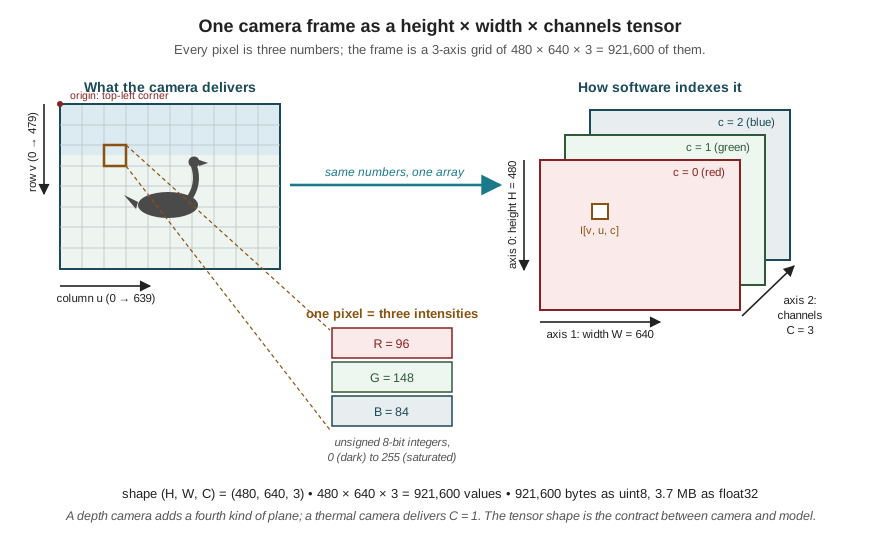
The shape is also a bill, and it is worth paying in full once. As delivered — one byte per value — a frame costs
\[ \begin{aligned} 480 \times 640 \times 3 &= 921{,}600\ \text{values} = 921{,}600\ \text{bytes} \approx 0.92\ \text{MB},\\ \text{at 30 frames/s:}\quad 921{,}600 \times 30 &\approx 27.6\ \text{MB/s}. \end{aligned} \]
That 27 MB/s is the same number Part I used to prove the imagery cannot leave the aircraft; it now reappears as the load the onboard pipeline must absorb continuously. And the bill grows before the model ever sees the frame: networks compute in floating point, and converting each 1-byte integer to a 4-byte float32 quadruples the footprint to about 3.7 MB per frame. Multiply by the buffering a real pipeline needs — the frame being captured, the frame being processed, the intermediate results — and image memory starts to compete for the companion computer’s RAM in earnest. The source constraint the next chapter makes precise is already visible in outline: in an embedded vision system, the activations — the tensors flowing between layers — often cost more memory than the model’s own weights, and every one of them scales with the input resolution chosen here.
The channel axis is where the tensor view starts earning its generality. Nothing about axis 2 says “colour”; it says “measured quantities per pixel,” and the running example’s Intel RealSense D455 makes the point physically. Alongside the RGB stream it produces a depth stream — a plane of the same spatial layout whose value at \((v, u)\) is the measured range, in millimetres, to whatever surface that pixel sees, delivered as 16-bit integers because 256 levels cannot span centimetre precision over tens of metres. Aligned to the colour frame, depth is simply a fourth channel a pipeline may stack on: \(C = 4\), shape 480 × 640 × 4. A thermal camera delivers \(C = 1\) — one radiometric plane. The tensor formalism absorbs all of these without modification, which is exactly why every vision framework speaks it.
Two bookkeeping conventions complete the picture, and both bite in practice. First, axis order: cameras and OpenCV deliver channels-last (\(H, W, C\) — the three colour values of one pixel adjacent in memory), while PyTorch expects channels-first (\(C, H, W\) — each colour plane contiguous), so every pipeline contains an explicit transpose, and supplying the wrong order fails silently or loudly but never correctly. Second, the batch axis: models process inputs in batches, adding a leading axis \(N\) for “which image,” so the tensor a PyTorch model actually receives is rank-4 with shape \((N, C, H, W)\) — for onboard inference, almost always \(N = 1\). A short exchange with a live frame makes all of this concrete:
import cv2
import numpy as np
import torch

frame = cv2.imread("field_frame.png")     # any 640x480 capture
print(frame.shape, frame.dtype)           # (480, 640, 3) uint8  -- H, W, C
print(frame[240, 320])                    # centre pixel, e.g. [ 84 148  96]
print(frame.nbytes)                       # 921600 bytes

x = torch.from_numpy(frame).float() / 255.0   # uint8 -> float32 in [0, 1]
x = x.permute(2, 0, 1).unsqueeze(0)           # (H,W,C) -> (1, C, H, W)
print(x.shape)                            # torch.Size([1, 3, 480, 640])
print(x.element_size() * x.nelement())    # 3686400 bytes -- the float bill
(One trap for the record: OpenCV orders the channels blue–green–red for historical reasons, so frame[240, 320] above prints B, G, R — a pipeline mixing OpenCV capture with a model trained on RGB images must swap channels explicitly, and this single silent mismatch has degraded more deployed detectors than any exotic failure.)
13.5 Spatial Structure: Why the Grid Is Not Just a List
A 480 × 640 × 3 tensor holds 921,600 numbers, and nothing so far prevents treating it as a flat vector of that length — forgetting the grid, keeping the values. What would be lost? Everything, and the argument is worth making precisely, because it is the founding argument of convolutional processing.
Consider a thought experiment. Take every frame the camera will ever produce and shuffle its pixels by one fixed permutation — the same scrambling applied to every frame. No information is destroyed: the permutation is invertible, and every pixel value survives. Yet the scrambled frames are meaningless to the eye, because what the eye reads is not the set of values but their arrangement: an edge is a coherent intensity change between neighbouring pixels, a texture is a repeating local pattern, a goose is a particular composition of curves and contrasts spanning a compact region. Adjacent pixels sample adjacent patches of the physical world, so nearby values are strongly correlated and jointly meaningful in a way that distant values are not. That is spatial structure, and the shuffle preserves the data while annihilating it.
Now count what ignoring it costs. The generic way to wire a flattened image into a network is a fully-connected layer: every input value connected, with its own weight, to every unit of the next layer. Even a modest first layer of 1,000 units costs
\[ \begin{aligned} 921{,}600 \times 1{,}000 &= 9.216 \times 10^{8}\ \text{weights} \\ \text{at 4 bytes each:}\quad &\approx 3.7\ \text{GB}, \end{aligned} \]
which is essentially the Jetson Nano’s entire 4 GB of memory spent before the network has a second layer — for a layer that, by construction, could learn the scrambled images exactly as easily as the real ones, because it assigns independent weights to every position and encodes no notion of “neighbouring.” Worse, whatever it learns it learns per location: the weights that come to recognize a goose centred in the frame say nothing about a goose near the edge, so every appearance position must be learned separately, from separate examples. The fully-connected layer is simultaneously too large to fit and too weak to generalize, and both failures have the same cause — it treats the image as a list.
The repair is to process the image the way its structure suggests: locally, and identically everywhere. A convolution takes a small grid of weights — a kernel, typically 3 × 3 per channel — and slides it across the image. At each position, the kernel is multiplied element-wise with the window of pixels beneath it and the products are summed to a single number; sliding over all positions produces a new plane, the feature map, aligned with the image, whose value at each location measures how strongly the kernel’s pattern is present there. Figure 13.2 traces one position through the operation with a classic hand-designed kernel that responds to vertical edges; in a network the kernel’s weights are not designed but learned, exactly as Part II’s reader learned that a PID gain is tuned rather than guessed — the mechanism is fixed, the numbers come from data.
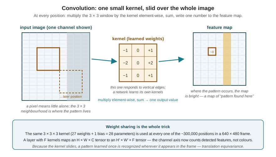
The arithmetic reverses spectacularly. A 3 × 3 kernel spanning all three input channels holds \(3 \times 3 \times 3 = 27\) weights plus one bias — 28 parameters — and those same 28 numbers examine every one of the roughly 300,000 window positions in the frame. Against the fully-connected layer’s \(9 \times 10^8\) weights, that is a reduction of seven orders of magnitude, purchased by an assumption the thought experiment just validated: the patterns that matter are local, and a pattern worth detecting at one position is worth detecting at every position. The second half of that assumption buys the generalization the flat layer lacked — because the kernel slides, a goose-shaped response learned from geese in the training set’s frame centres fires just as well on a goose in the corner. The property is called translation equivariance: shift the input, and the feature map shifts with it, rather than the detection failing.
One kernel yields one feature map, and one pattern detector does not make a perception system, so a convolutional layer learns a bank of \(F\) kernels and stacks their maps: an \(H \times W \times C\) input becomes an \(H' \times W' \times F\) output. Read that shape carefully, because it is the moment the tensor formalism pays for itself: the output is again a rank-3 tensor of the same form as the input, but its channel axis no longer counts colours — it counts features found. Layer two convolves over layer one’s feature maps and finds patterns of patterns; by the depth of a real network the channels encode fragments like “textured round body” and “long curved neck,” still organized on a spatial grid that remembers where. Every tensor between the camera and the answer has the same three-axis anatomy established in Figure 13.1 — which is why this chapter’s representation, and not any particular network, is the true foundation of Part III. How many layers, how many kernels, and how the whole stack is trained and squeezed into the Jetson’s power budget is the business of the next chapter, on TinyML; what cannot change, whatever those answers are, is the shape of the data flowing through.
13.6 Three Tasks, One Tensor
Everything so far concerns the input. The output side has its own taxonomy, and choosing from it is a mission decision, not a modelling detail. Inference — running the trained model forward on a live frame — always consumes the same \((1, 3, H, W)\) tensor; what distinguishes the classical vision tasks is the structure of what comes back. Figure 13.3 puts the three that matter for this book side by side on the same scene.
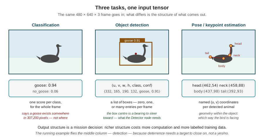
Classification answers one question about the whole frame: which class is this? The model’s final output is a vector of scores, one per class — here perhaps just two, goose and no goose — normalized so they read as confidences. It is the least structured output, the cheapest to compute, and the cheapest to train, because labelling a training image requires only a word. Its limitation is exactly its economy: a classification of the running example’s frame asserts that a goose exists somewhere in 307,200 pixels. For a wildlife survey counting animals in archived imagery frame by frame, that can suffice. For a vehicle that must close on the animal, it is a fact without a direction.
Object detection answers what is present, and where — for every instance. The output is a variable-length list: for each object found, a bounding box — an axis-aligned rectangle, parameterized as a centre \((u, v)\) with width and height, or equivalently by two corners, in pixel coordinates — plus a class label and a confidence. The structural leap from classification is real and it is the reason detection is harder to train and to run: the model must produce zero, one, or many answers per frame, each tied to a location, and its training data must contain drawn boxes, not just words. (The loss that trains such a model correspondingly combines a classification term, a box-geometry term, and a confidence term — a composite the next chapters return to; for now the point is that output structure dictates training structure.)
Pose estimation — keypoint detection — answers how the object is arranged: it locates named structural points as pixel coordinates, head and neck-base and tail for a bird, joints for a person. It recovers geometry within the object that a box discards — which way the animal faces, whether wings are spread — at the price of still more computation and far more expensive labels, every training image needing every keypoint clicked.
The running example needs the middle column, and it is worth stating the reasoning as engineering rather than as taste, because the Building a Detection Pipeline chapter builds directly on it. The deterrence behavior of Part II’s state machine needs a target to steer toward: a direction, updated at frame rate. A detection’s box centre \((u, v)\) provides exactly that — through camera geometry, a pixel position is a bearing from the camera — and this is where the D455’s fourth channel closes the loop Part I promised: the depth value at that same \((v, u)\) supplies the missing range, and bearing plus range is a 3D target position in the vehicle’s frame. That triple — detect, look up depth, transform — is the target-position topic the mission logic has consumed since Part II, finally traced back to its pixels. Classification cannot feed it, for want of a location. Pose estimation could enrich it — a bird’s heading would help predict its escape direction — but it costs compute the Jetson’s budget will be shown (next chapter) to need elsewhere, and the deterrence maneuver as designed needs a position, not a posture. Richer output structure is bought with computation and labelled data; buy what the mission needs.
13.6.1 Pixels on target
One more quantity binds the input representation to the task, and it was promised in Part I: the search altitude is “fixed from below by the pixels-on-target requirement.” That requirement can now be computed. The Commercial Drone Landscape chapter’s ground-sample-distance relation, \(\text{GSD} = pH/f\), says one pixel spans a ground distance set by pixel pitch, height, and focal length; the ratio \(p/f\) is just the angle one pixel subtends, so for a camera viewing a target at range \(R\) the same relation reads: one pixel covers \(R \, \theta_{\text{pix}}\) metres, where \(\theta_{\text{pix}}\) is the per-pixel angle. The D455’s colour camera spans a horizontal field of view of about \(90^\circ\); in the 640-column mode,
\[ \theta_{\text{pix}} = \frac{90^\circ}{640} = 0.141^\circ = 2.45\ \text{mrad per pixel}. \]
A Canada goose’s body is roughly 0.35 m long. At a range of 20 m,
\[ \begin{aligned} \text{metres per pixel} &= R\,\theta_{\text{pix}} = 20 \times 2.45\times 10^{-3} = 4.9\ \text{cm} \\ \text{pixels on goose} &= \frac{0.35}{0.049} \approx 7\ \text{pixels}; \end{aligned} \]
at 10 m the same goose spans about 14 pixels. Seven pixels is a smudge — a detector fed smudges produces confidences barely above its false alarms — while double that begins to be a bird, with a visible neck and body to compose features from. The number explains, quantitatively, why the running example’s search leg flies at a few tens of metres and not at the legal ceiling, and it plants a warning the preprocessing section is about to pay off: resolution spent at the camera can be silently un-spent before the model ever sees the frame.
13.7 From Camera Frame to Model Input
Between the USB cable and the network sits a short, unglamorous, load-bearing stage the source pipeline names in one word: preprocess — resize, crop, normalize. A trained network’s first layer has a fixed input shape, almost never the camera’s: detection models commonly expect a square input such as 640 × 640 or smaller, chosen (next chapter) to fit a compute budget. The camera’s 640 × 480 frame must be resized to that shape — and because 640 × 480 is not square, either non-uniformly stretched (distorting every goose) or, standardly, scaled uniformly and padded with dead bands to fill the square (letterboxing), in which case every box the detector reports lives in the model’s coordinates and must be mapped back through the same scale and offset before it means anything in camera pixels. An alternative to shrinking everything is cropping a region of interest: once a target is being tracked, feeding the model a full-resolution crop around its last known position spends the whole input budget where the target is — more pixels on goose from the same camera — at the risk that a second bird outside the crop goes unseen. Finally the values are normalized — converted to float and scaled to \([0,1]\), often further shifted and scaled per channel to match the statistics the network was trained under — and the axes transposed to \((1, C, H, W)\), exactly the permute/unsqueeze lines of the earlier code block.
The resize step deserves respect rather than habit, because it is where this chapter’s threads knot together. Computation and activation memory both scale with the pixel count of the model’s input — halve each side and both fall by four, which is the single most powerful lever the next chapter has for fitting perception into the Jetson’s budget. But the pixels-on-target arithmetic runs on the resolution the model sees, not the resolution the sensor captured: downsample a frame in which a goose spans 14 pixels by two, and the detector receives a 7-pixel smudge — the camera’s resolution silently discarded in a line of preprocessing. Input resolution is thus a genuine design variable with a constraint from each side: pushed down by power, memory, and frame-rate, pushed up by detection range at mission altitude. Setting it is not a preprocessing detail; it is the first negotiation between this chapter’s representation and the next chapter’s constraints, and the Building a Detection Pipeline chapter will settle it with measurements rather than defaults.
That is the foundation laid. An image is a tensor; the tensor’s grid carries the spatial structure that convolution — a few shared weights, slid everywhere — is shaped to exploit; feature maps carry that structure through a network, layer by layer, in the same three-axis form; and out the far end comes an answer whose structure was a mission decision, made here: the running example detects, because deterrence needs a bearing. What remains is everything the word trained has been holding back — how the kernels’ numbers are learned, and how a network of them is compressed until it runs, at frame rate, inside a 10-watt computer bolted to a 2.2-kilogram aircraft. That is TinyML, and it is the next chapter.
13.8 Check Your Understanding
- The running example is considered for an upgrade to a camera mode of 1280 × 720 at 30 frames/s. Compute the per-frame memory as delivered (uint8, 3 channels) and after conversion to
float32, and the raw delivered data rate. State one quantity in the perception pipeline that this upgrade quadruples besides the frame itself.
Per frame: \(720 \times 1280 \times 3 = 2{,}764{,}800\) values — about 2.76 MB as uint8, and \(\times 4 = 11.1\) MB as float32. At 30 frames/s the camera delivers \(2{,}764{,}800 \times 30 \approx 83\) MB/s, three times the 640 × 480 mode’s ~27.6 MB/s. Beyond the frame itself, the activations — the feature-map tensors between network layers — scale with input pixel count, so if the model’s input resolution is raised to exploit the new camera, every layer’s activation memory and compute grow in proportion (quadrupling if both input sides are doubled). A sharper camera whose frames are downsampled back to the old model input, by contrast, buys nothing at all.
- Every frame the camera produces is scrambled by the same fixed, invertible pixel permutation before being stored. Exactly as much information survives as before. Explain why a fully-connected network could in principle learn to classify the scrambled frames as well as the originals, why a convolutional network could not, and what this asymmetry reveals about what convolution assumes.
A fully-connected layer assigns an independent weight to every input position and encodes no notion of neighbourhood; relabelling the positions (which is all a fixed permutation does) just relabels the weights, so its learning problem is unchanged. A convolutional network, by contrast, hard-codes the assumption that meaningful patterns are local — its kernels only ever see small contiguous windows — and the permutation destroys locality: pixels that were neighbours in the world are scattered across the grid, so no small window contains a coherent pattern to detect. The asymmetry shows that convolution is not a generic function approximator but a structural commitment: it wins on images precisely because, and only because, images really do concentrate their meaning in local spatial arrangements. Where that assumption fails, so does the architecture’s advantage.
- Compute the parameter count of (a) a fully-connected layer from a flattened 480 × 640 × 3 image to 1,000 units, and (b) a convolutional layer of 32 kernels, each 3 × 3 spanning all 3 input channels, with one bias per kernel. State the output tensor shape of (b) (assume the spatial size is preserved) and what its channel axis now means.
- \(921{,}600 \times 1{,}000 = 9.216 \times 10^8\) weights (plus 1,000 biases) — about 3.7 GB in float32. (b) Each kernel holds \(3 \times 3 \times 3 = 27\) weights plus 1 bias, so 32 kernels hold \(32 \times 28 = 896\) parameters — six orders of magnitude fewer, independent of image size. The output shape is \(480 \times 640 \times 32\): one feature map per kernel, spatially aligned with the input. The channel axis no longer indexes colours but features — each of the 32 planes maps where one learned local pattern occurs in the frame.
- For each requirement, name the vision task (classification, detection, or pose estimation) whose output structure is the minimum sufficient, and say what the output supplies that the next-cheaper task cannot. (a) Post-flight review flags which archived frames contain any goose, for a human to audit. (b) The deterrence behavior steers toward the nearest goose in view. (c) A researcher asks whether deterred geese take off away from the aircraft’s approach direction.
- Classification — a per-frame label and confidence is exactly the required output; location within the frame is unused because a human will look at flagged frames anyway. (b) Detection — steering needs a per-instance location; the box centre gives a bearing (and, with the depth channel, a range), and “nearest” requires distinguishing instances, which a whole-frame label cannot do. (c) Pose estimation — take-off direction relative to approach requires the animal’s orientation, geometry within the object; a bounding box records extent but not which end is the head, so detection cannot answer it. The pattern: each step up buys structure — location, then internal geometry — and should be bought only when the mission question actually consumes it.
- Using the chapter’s numbers (90° across 640 columns, goose body 0.35 m), find the maximum range at which a goose still spans at least 15 pixels. The pipeline then letterboxes the 640-wide frame into a 320 × 320 model input. What does the effective per-pixel angle become, and what happens to your range?
At \(\theta_{\text{pix}} = 2.45\) mrad, the goose spans \(0.35/(R \times 2.45\times10^{-3})\) pixels; setting that to 15 gives \(R = 0.35/(15 \times 2.45\times10^{-3}) \approx 9.5\) m. Letterboxing 640 columns into 320 halves the horizontal pixel count across the same 90° field, so the effective per-pixel angle doubles to 4.9 mrad — and the 15-pixel range halves to about 4.8 m. The camera did not change; a preprocessing line halved the detection range. This is why input resolution is negotiated against the mission’s required detection range, not defaulted — and why the running example’s search altitude and its model input size are coupled decisions.
- The detection pipeline reports a goose with box centre \((u, v) = (400, 300)\) in the 640 × 480 colour frame. Part I claimed the depth camera “earns its mass” at this moment. State precisely what the detector’s output alone determines about the goose’s position, what single additional lookup the aligned depth stream provides, and why a monocular (colour-only) camera would instead have to maneuver to recover the same information.
The box centre fixes only a direction: through the camera geometry, pixel \((400, 300)\) corresponds to a ray from the camera — a bearing — with the goose lying somewhere along it at unknown range; a nearby goose and a distant large object can produce the same pixels. The aligned depth stream turns position into one array lookup: the depth value at \((v, u) = (300, 400)\) is the range along that ray, and bearing plus range fixes the goose’s 3D position in the vehicle’s frame — the content of the target-position topic the mission logic consumes. A monocular camera measures no range, so it would have to triangulate: observe the goose from two or more separated viewpoints and intersect the bearings, which costs maneuvering time against a moving animal and couples perception accuracy to flight precision. The depth camera converts that flight problem into memory access.
13.9 Try It
Part 1 — hold the tensor in your hands. Take any outdoor photograph (a field with birds is ideal; failing that, any scene with a distinct subject) and open it in Python with OpenCV or PIL. Verify the claims of this chapter against it one by one: print the shape and dtype and identify \(H\), \(W\), and \(C\); index a pixel you can point to in the image and check the value ordering (is it RGB or BGR?); split and display the three channel planes separately and find a feature visible in one channel but weak in another. Then run the chapter’s thought experiment for real: build one fixed random permutation, apply it to the pixels, and display the result — then invert it and confirm the image returns. Finally, downsample the image by factors of 2, 4, 8, and 16 and find the factor at which you can no longer identify the subject; measure the subject’s size in pixels at that scale. You have just located your own pixels-on-target threshold — keep the number in mind when a detector’s is discussed.
Part 2 — convolve by hand, then size the mission. Implement 2D convolution yourself in a dozen lines of NumPy — loops are fine, clarity over speed — and apply the vertical-edge kernel from Figure 13.2 and its transpose to a grayscale version of your image. Display both feature maps and check they are bright where you predicted. Convince yourself of translation equivariance: shift the input a few pixels, re-convolve, and compare. Then put the chapter’s last relation to work for the running example: tabulate metres-per-pixel and pixels-on-goose (0.35 m body) at ranges of 5, 10, 20, and 40 m for the 640-column mode, and repeat for model input widths of 640, 416, and 320 after letterboxing. Pick the lowest model resolution that still keeps at least 15 pixels on a goose at your chosen search range, and write two sentences defending the choice — one about detection, one about what the saved computation buys, which the next chapter will make quantitative.
Related Lab: See Appendix B for the lab assignment that applies this chapter’s concepts.