18 Coordinate Frames: From Camera to World
Part III ended with a detector that works: a network on the companion computer that draws a box around a goose, and a depth camera whose aligned range image turns that box’s centre into a distance. The Building a Detection Pipeline chapter was explicit about what those two numbers buy — the box centre fixes a bearing, the depth value fixes a range along it, and together they pin the goose’s position in three dimensions. What that chapter deliberately left unexamined is the fine print on the word position. Position relative to what? The camera reports the goose relative to its own lens, in axes that tilt every time the airframe rolls and pivot every time it yaws. The autopilot, meanwhile, accepts Offboard setpoints in the local North-East-Down frame introduced in the PX4 Autopilot Stack chapter — axes nailed to the world, origin frozen at the launch point — and that chapter promised that the frame conventions behind its “z is down, so altitude is negative” sign discipline would get a chapter of their own in Part IV. This is that chapter.
The gap it closes is not a technicality. A detection expressed in camera coordinates is unusable as a navigation target: “6 metres out along the lens axis” means a different world location every few milliseconds as the aircraft moves, and handing it raw to the flight controller would command the drone toward wherever its own nose happens to point. Between the perception system and the navigation system there must sit a piece of mathematics — small, exact, and utterly load-bearing — that re-expresses the same physical point in the world’s coordinates. In the running example that mathematics lives in one module, frames.py, whose entire public surface is eight short functions; this chapter derives what those functions compute. The material is the first genuinely geometric machinery of the book, and it will be spent again immediately: every planner in this Part consumes targets and waypoints in the NED frame this chapter learns to reach.
18.1 Learning Objectives
- Name the three coordinate frames a vision-guided drone must reconcile — camera optical, body FRD, and local NED — and state each frame’s axis convention, what it is attached to, and why no two of them can be conflated.
- Derive the optical-to-body transformation for a forward-facing camera as an axis remapping composed with a mounting-pitch rotation, and verify that the remapping is a proper rotation rather than a reflection.
- Convert a PX4 attitude quaternion into a rotation matrix, and explain why quaternions rather than Euler angles carry the attitude across the body-to-NED step.
- Carry a real detection numerically through the complete chain — pixel and depth to camera point, to body frame, to relative NED, to absolute NED — and sanity-check the result against physical expectations.
- Express the full pipeline as a product of homogeneous transformations, and quantify the dominant error sources — extrinsic calibration, attitude error, synchronization latency, and depth uncertainty — as position error at the mission’s working ranges.
18.2 Key Vocabulary
- Camera optical frame — the coordinate frame attached to the camera lens under the ROS REP-103 convention: x to the right of the image, y downward in the image, z forward along the viewing direction; the frame in which a depth camera reports every detected point.
- FRD (Forward-Right-Down) — PX4’s body frame convention: x out the nose, y out the right side, z down through the belly; attached to the airframe and rotating with it, so a fixed world point has constantly changing FRD coordinates in flight.
- NED (North-East-Down) — the local world frame in which PX4 navigates: x North, y East, z Down, origin at the point where the state estimator initialized (the launch point); the frame of every Offboard position setpoint, where altitude appears as negative z.
- Rotation matrix — a 3 × 3 orthogonal matrix with determinant +1 that re-expresses a vector in a rotated frame without changing its length; its inverse is its transpose, which makes reversing any frame transformation computationally free.
- Quaternion — a four-component representation of 3D orientation, written \([w, x, y, z]\) in PX4’s convention, that encodes an axis and an angle of rotation without the singularities of three-angle representations; the native attitude output of the flight controller’s estimator.
- Gimbal lock — the degeneracy of Euler-angle representations in which two of the three rotation axes align (at ±90° pitch), collapsing a degree of freedom; the classical argument for carrying attitude as a quaternion.
- Homogeneous transformation — a 4 × 4 matrix \(T = \begin{bmatrix} R & t \\ 0 & 1 \end{bmatrix}\) packaging a rotation and a translation so that chains of frame changes compose by ordinary matrix multiplication.
- Camera intrinsics — the parameters of the camera’s own projection (focal lengths \(f_x, f_y\) and principal point \(c_x, c_y\), in pixels) that convert between a pixel coordinate and a direction in the optical frame.
- Extrinsic calibration — the fixed rigid transform between the camera and the airframe — where the camera sits and how it is tilted — measured once at build time; an error here biases every detection the system will ever make, in the same direction.
18.3 One Point, Three Frames
Every sensor bolted to an aircraft measures in its own private coordinate system, and before any two measurements can be combined — or a measurement handed to a controller — they must be re-expressed in a common frame. The running example’s navigation pipeline threads exactly three. Figure 18.1 draws them side by side, and the differences among them are worth reading closely, because each difference is a transformation the software must perform.
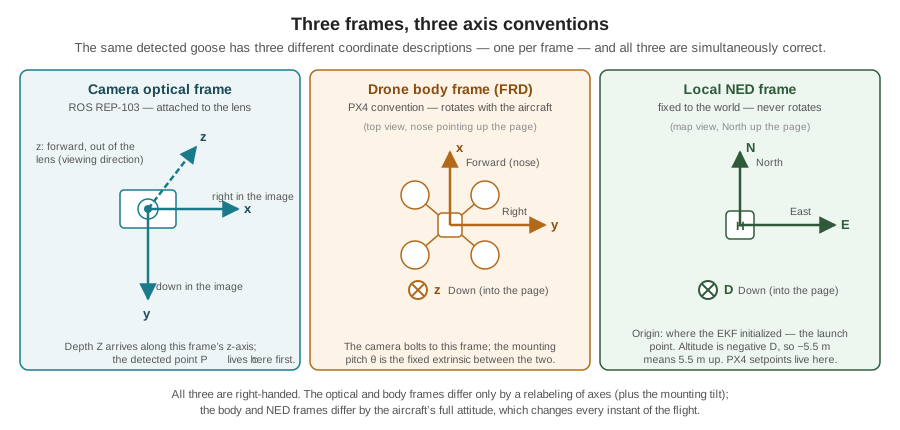
The camera optical frame is the convention ROS standardizes in REP-103 and the one the running example’s Intel RealSense reports in: x points to the right of the image, y points down the image, and z points out of the lens along the viewing direction. The choice looks eccentric until it is set beside the image-coordinate convention from the Images as Data chapter — column index \(u\) increasing rightward, row index \(v\) increasing downward from a top-left origin. The optical frame is that screen convention extruded into 3D: x tracks \(u\), y tracks \(v\), and z carries the one thing a depth camera adds, range outward. A detected goose enters the pipeline as a point in this frame,
\[ P_C = \begin{bmatrix} x_C \\ y_C \\ z_C \end{bmatrix}, \]
and getting from the detector’s actual output — a pixel and a depth — to \(P_C\) is the projection geometry that chapter deferred. A pinhole camera maps a 3D point to the pixel \(u = f_x \, (x_C / z_C) + c_x\), where \(f_x\) is the focal length measured in pixels and \(c_x\) the image centre; run backward, with the depth value supplying \(z_C = Z\) directly (the RealSense reports perpendicular distance to the image plane, not slant range):
\[ x_C = \frac{(u - c_x)\, Z}{f_x}, \qquad y_C = \frac{(v - c_y)\, Z}{f_y}. \]
The intrinsics come from the camera’s factory calibration, but a serviceable estimate falls out of geometry: a 90° horizontal field of view spread across 640 columns means the 320 columns on either side of centre span 45°, so \(f_x = 320/\tan 45^\circ = 320\) pixels. Take the goose the Images as Data chapter boxed at \((u, v) = (400, 300)\) in the 640 × 480 frame, and let the aligned depth lookup at that pixel return 6.00 m:
\[ \begin{aligned} x_C &= \frac{(400 - 320)(6.00)}{320} = 1.50\ \text{m} \\ y_C &= \frac{(300 - 240)(6.00)}{320} \approx 1.13\ \text{m} \\ P_C &= [\,1.50,\ 1.13,\ 6.00\,]\ \text{m}. \end{aligned} \]
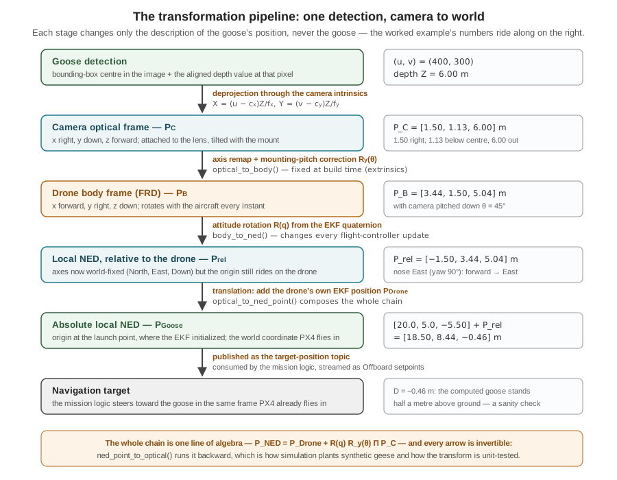
The goose sits 6 m out along the lens axis, 1.5 m to the right of it, 1.13 m below it. That is a complete, correct 3D position — and it is useless to the autopilot, because every one of those numbers is measured against a lens that moves.
The drone body frame is PX4’s FRD convention: x forward out the nose, y right, z down. It is rigidly attached to the airframe and rotates with it. The camera is bolted to this frame — in the running example, tilted downward so the search pattern’s forward flight keeps the ground in view — so the relationship between optical and body coordinates is fixed at build time: a constant rotation, part of the system’s extrinsic calibration, that never changes in flight.
The local NED frame is the one the reader has been flying in since Part II: x North, y East, z Down, origin wherever the flight controller’s state estimator initialized — the launch point, which is why the very first Offboard example commanded -5.0 to mean five metres up. Unlike the other two frames it never rotates; it is the closest thing the system has to “the world.” Every position the autopilot publishes, and every setpoint it accepts, lives here.
Three frames, and two fundamentally different kinds of separation between them. Optical-to-body is a constant transform, knowable in advance to whatever precision the tape measure and the mounting jig allow. Body-to-NED is the aircraft’s attitude — it changes with every gust and every commanded turn, and no measurement made at build time can supply it. Something on the aircraft must estimate it continuously, and something does: the flight controller’s EKF, whose construction from gyroscope, accelerometer, and magnetometer evidence the Sensing the World chapter told in full. This chapter does not reopen that story. It stands on its result — the estimator publishes the vehicle’s attitude, as a quaternion, many times per second — and asks only what to do with it.
18.4 The Pipeline in One Equation
The complete journey from detection to navigation target is a single line of algebra:
\[ P_{NED} \;=\; P_{Drone} \;+\; R^{NED}_{Body}\, R^{Body}_{Camera}\, P_{Camera}. \]
Read it right to left, the order in which the operations act. \(P_{Camera}\) is the detected point in the optical frame — the \([1.50, 1.13, 6.00]\) just computed. \(R^{Body}_{Camera}\) is the fixed extrinsic rotation that re-expresses it in the body frame; the superscript–subscript notation names the frames, “from Camera coordinates into Body coordinates.” \(R^{NED}_{Body}\) is the attitude rotation, built fresh from the EKF’s current quaternion, that re-expresses the body-frame vector in world axes. At that point the vector is world-aligned but still measured from the aircraft — a displacement, “the goose is 3.4 m East of me” — so the final step adds \(P_{Drone}\), the drone’s own EKF position, translating the origin from the aircraft to the launch point. Rotations first, translation last: rotations act on directions, and only after the directions are world-aligned does adding a world-frame position make sense. Figure 18.2 lays the chain out stage by stage, with the worked example’s numbers riding alongside; the two sections that follow derive its two rotations.
18.5 Optical to Body: A Relabeling and a Tilt
Suppose first that the camera is mounted perfectly level, looking straight out the nose. Then the optical and body frames are the same physical directions wearing different labels, and the transformation is pure bookkeeping. Where does the camera’s z-axis point? Out of the lens — which is out of the nose: the body’s x. Where does the camera’s x point? Right in the image — the body’s y. The camera’s y? Down the image — the body’s z. Three questions, three answers, and the transformation is written:
\[ x_B = z_C, \qquad y_B = x_C, \qquad z_B = y_C, \]
or as a matrix acting on \(P_C\),
\[ \Pi \;=\; \begin{bmatrix} 0 & 0 & 1 \\ 1 & 0 & 0 \\ 0 & 1 & 0 \end{bmatrix}, \qquad P'_B = \Pi\, P_C . \]
\(\Pi\) deserves one check before it is trusted: is it a rotation? Its columns are orthonormal, and its determinant is \(+1\) — it is the cyclic permutation \((x, y, z) \to (z, x, y)\), and cyclic permutations of a right-handed triad are genuine rigid rotations. Had the mapping instead swapped exactly two axes, the determinant would be \(-1\): a reflection, which no physical mounting of a rigid camera can produce. A determinant check is thirty seconds of arithmetic that catches an entire class of frame bugs — coordinate systems accidentally mirrored — that otherwise surface as a drone that turns left toward geese on its right.
Real mountings are not level. The running example’s camera is pitched downward by a fixed angle \(\theta\) so that forward flight sweeps the ground; that tilt is a rotation about the body’s y-axis, applied after the relabeling:
\[ R_y(\theta) = \begin{bmatrix} \cos\theta & 0 & -\sin\theta \\ 0 & 1 & 0 \\ \sin\theta & 0 & \cos\theta \end{bmatrix}, \qquad P_B = R_y(\theta)\, P'_B . \]
Sign conventions in rotation matrices are where frame code quietly goes wrong, so verify this one physically rather than trusting it. A goose dead ahead of the camera at distance \(d\) has \(P'_B = [d, 0, 0]\) after relabeling. If the camera is tilted down by \(\theta\), that goose is really below the aircraft’s horizontal plane — forward and down. Apply the matrix: \(R_y(\theta)\,[d, 0, 0]^T = [\,d\cos\theta,\ 0,\ d\sin\theta\,]^T\). Forward component \(d\cos\theta\), downward component \(d\sin\theta\) — positive z, and z is down in FRD. The matrix passes: positive \(\theta\) means a downward-looking camera, exactly the convention the mounting drawing uses. Together, \(R^{Body}_{Camera} = R_y(\theta)\,\Pi\), the fixed extrinsic rotation of the master equation.
Now run the worked example through, with the camera pitched down \(\theta = 45^\circ\) (\(\cos\theta = \sin\theta \approx 0.7071\)). Relabeling first:
\[ P'_B = \Pi \begin{bmatrix} 1.50 \\ 1.13 \\ 6.00 \end{bmatrix} = \begin{bmatrix} 6.00 \\ 1.50 \\ 1.13 \end{bmatrix}, \]
then the tilt:
\[ \begin{aligned} x_B &= 0.7071\,(6.00) - 0.7071\,(1.13) = 0.7071 \times 4.87 \approx 3.44 \\ y_B &= 1.50 \\ z_B &= 0.7071\,(6.00) + 0.7071\,(1.13) = 0.7071 \times 7.13 \approx 5.04 \\ P_B &= [\,3.44,\ 1.50,\ 5.04\,]\ \text{m}. \end{aligned} \]
The goose is 3.44 m ahead of the aircraft, 1.50 m to its right, and 5.04 m below it. Notice what the tilt did: most of what the camera called “forward” became, in the body’s honest axes, depth below the aircraft — which is exactly what a 45°-down camera looking at a ground target should report.
18.6 Body to NED: The Quaternion Does the Work
The second rotation cannot be measured with a jig, because it is the aircraft’s attitude and it changes continuously. The flight controller’s estimator publishes it as a unit quaternion \(q = [w, x, y, z]\) — four numbers with \(w^2 + x^2 + y^2 + z^2 = 1\), encoding a single axis in space and a single angle of rotation about it (via \(w = \cos(\alpha/2)\), with \([x,y,z]\) the rotation axis scaled by \(\sin(\alpha/2)\)). The standard expansion converts it to the rotation matrix that carries body-frame vectors into NED:
\[ R(q) = \begin{bmatrix} 1 - 2(y^2 + z^2) & 2(xy - wz) & 2(xz + wy) \\ 2(xy + wz) & 1 - 2(x^2 + z^2) & 2(yz - wx) \\ 2(xz - wy) & 2(yz + wx) & 1 - 2(x^2 + y^2) \end{bmatrix}, \qquad P^{rel}_{NED} = R(q)\, P_B . \]
Why a quaternion, when three Euler angles — roll, pitch, yaw — seem so much more legible? Four reasons, in ascending order of practical weight. Singularity: Euler angles represent attitude as three chained rotations, and at ±90° pitch two of the three axes align — gimbal lock — collapsing a degree of freedom, so the representation cannot even express which way the vehicle is turning; an acrobatic or wind-thrown multirotor visits that neighborhood, and estimator mathematics must not blow up when it does. Numerical stability: accumulated floating-point error pushes a quaternion slightly off unit length, and the fix is one renormalization — divide four numbers by their norm — whereas a drifting 3 × 3 matrix must be re-orthogonalized, an expensive and delicate repair. Interpolation: blending smoothly between two attitudes (needed whenever measurements must be aligned across time, as the error-budget section will want) is well defined for quaternions and badly behaved for Euler angles. And nativeness: the estimator the Sensing the World chapter described carries its attitude state as a quaternion; PX4 publishes it in exactly the \([w, x, y, z]\) order used here, so consuming it directly avoids a conversion — and every conversion between attitude conventions is an opportunity for a sign error that flies the aircraft somewhere surprising.
The matrix \(R(q)\), like every rotation matrix, is orthogonal: its inverse is its transpose. That property is worth pausing on because the software leans on it. Transforming a NED vector back to the body frame — which the mission logic needs whenever it asks “which way, in my own axes, is that world point?” — requires no matrix inversion at all, just \(R^T\), numerically exact and nearly free.
Put the worked example’s aircraft in a definite attitude: level flight, nose due East — a yaw of \(\psi = 90^\circ\), so \(q = [\cos 45^\circ, 0, 0, \sin 45^\circ] = [0.7071, 0, 0, 0.7071]\). Substituting \(w = z = 0.7071\), \(x = y = 0\) into \(R(q)\):
\[ R(q) = \begin{bmatrix} 0 & -1 & 0 \\ 1 & 0 & 0 \\ 0 & 0 & 1 \end{bmatrix}, \]
which reads as a sanity check in matrix form: body-forward \([1,0,0]\) maps to \([0,1,0]\) — East, where the nose points; body-right maps to \([-1,0,0]\) — South, which is indeed to the right of an eastbound aircraft; body-down maps to down. Applying it:
\[ P^{rel}_{NED} = R(q) \begin{bmatrix} 3.44 \\ 1.50 \\ 5.04 \end{bmatrix} = \begin{bmatrix} -1.50 \\ 3.44 \\ 5.04 \end{bmatrix}. \]
The goose is 3.44 m East of the drone, 1.50 m South of it (negative North), and 5.04 m below it — the same displacement as before, now expressed in axes that will not move when the aircraft does.
18.7 From Relative to Absolute
One step remains, and it is an addition. The vector just computed is world-aligned but drone-centred; the autopilot navigates toward absolute positions, measured from the EKF origin at the launch point. The drone knows its own position in that frame — the same estimate the Offboard examples of Part II consumed — so:
\[ P_{Goose} = P_{Drone} + P^{rel}_{NED}. \]
Give the worked example’s aircraft the position \(P_{Drone} = [20.0,\ 5.0,\ -5.50]\) — 20 m North and 5 m East of launch, at the 5.5 m mission altitude the Part II survey plan flew:
\[ P_{Goose} = \begin{bmatrix} 20.0 \\ 5.0 \\ -5.50 \end{bmatrix} + \begin{bmatrix} -1.50 \\ 3.44 \\ 5.04 \end{bmatrix} = \begin{bmatrix} 18.50 \\ 8.44 \\ -0.46 \end{bmatrix}. \]
And here the chain hands back its first reward: a physical sanity check. \(D = -0.46\) m puts the computed goose 0.46 m above the launch-pad ground plane — about the height of a standing goose’s body. Had a sign been wrong anywhere in the chain — the pitch matrix transposed, the quaternion order scrambled, the remap mirrored — this number would come out as a goose 10 m underground or hovering at altitude, and the error announces itself. Checking the D-component of transformed ground targets against “roughly zero” is the cheapest regression test the perception-to-navigation boundary has, and the running example’s integration tests use exactly it.
18.7.1 The Same Chain as One Matrix
The pipeline was derived as rotate, rotate, add — but there is a standard notation that folds all three steps into products of a single object, and it is the notation every robotics text and every ROS transform library speaks. Append a 1 to each position vector, \(\tilde{P} = [x, y, z, 1]^T\), and package each frame change as a 4 × 4 homogeneous transformation:
\[ T = \begin{bmatrix} R & t \\ \mathbf{0}^T & 1 \end{bmatrix}, \qquad T\,\tilde{P} = \begin{bmatrix} R P + t \\ 1 \end{bmatrix}. \]
The appended 1 is the whole trick: it multiplies the translation column \(t\), so a single matrix–vector product now performs rotate-and-translate. Chains of frames compose by plain matrix multiplication, in the same right-to-left reading order as before:
\[ \tilde{P}_{W} = T^{World}_{Drone}\; T^{Drone}_{Camera}\; \tilde{P}_C, \]
where \(T^{Drone}_{Camera}\) carries the extrinsic rotation \(R_y(\theta)\,\Pi\) together with the camera’s mounting offset from the vehicle centre (a few centimetres this chapter has quietly neglected — the homogeneous form is where it stops being neglectable), and \(T^{World}_{Drone}\) carries the attitude rotation \(R(q)\) together with \(P_{Drone}\). The subscript-cancellation reading — Camera cancels against Camera, Drone against Drone — makes long chains auditable at a glance, and inverting any link is mechanical: \(T^{-1} = \begin{bmatrix} R^T & -R^T t \\ \mathbf{0}^T & 1 \end{bmatrix}\). For a two-link chain the explicit form of this chapter and the homogeneous form are the same arithmetic; the homogeneous form wins the moment a third frame appears — a gimbal between camera and body, a second aircraft, a map frame above NED — which is precisely the direction this Part is headed.
18.8 The Module in Code
All of the above compiles down to remarkably little software. The running example’s frames.py exposes the two rotations, their inverses, and the composed chain — eight functions, each a few lines of NumPy:
| Function | Computes |
|---|---|
quat_to_rot(q) |
\(R(q)\): the body-to-NED rotation matrix from a PX4 \([w,x,y,z]\) quaternion |
optical_to_body(v, pitch) |
\(R_y(\theta)\,\Pi\,v\): axis remap plus mounting-pitch correction |
body_to_ned(v, q) |
\(R(q)\,v\): attitude rotation into world axes |
body_to_optical(v, pitch) / ned_to_body(v, q) |
the inverses, via transposes — no matrix inversion anywhere |
optical_to_ned_point(p, q, drone, pitch) |
the full chain: \(P_{Drone} + R(q)\,R_y(\theta)\,\Pi\,p\) |
ned_point_to_optical(p, q, drone, pitch) |
the full chain backward |
The composed forward function is the master equation verbatim:
def optical_to_ned_point(p_opt, q_wxyz, drone_ned, camera_pitch_rad=0.0):
    """Detected point (optical frame) -> absolute local NED position."""
    rel_ned = body_to_ned(optical_to_body(p_opt, camera_pitch_rad), q_wxyz)
    return np.asarray(drone_ned, dtype=float) + rel_ned
Two design choices in the module repay attention. First, every inverse is computed by transpose, never by np.linalg.inv — the orthogonality of rotation matrices, cashed in as both speed and numerical exactness. Second, the module ships its own inverse chain, ned_point_to_optical(), whose stated consumers are simulation and testing: plant a synthetic goose at a known NED position, run the inverse chain to compute what the camera should see, feed that to the pipeline as a fake detection, and the forward chain must reproduce the planted position to machine precision, for randomized attitudes and camera angles. A transform library that round-trips thousands of random points is trustworthy in a way no amount of staring at sign conventions can establish — geometry code fails silently, so it must be tested loudly.
Where this module sits in the running system is a story for later: the Systems Architecture chapter in Part V draws the full ROS 2 node graph, with the frame conversion living between the Detector’s camera-frame output and the Mission Manager’s world-frame target topic — the position it must occupy, since it is the only component that consumes both the perception stream and the flight controller’s state estimate at once.
18.9 Where the Centimetres Go
The derivations above are exact; the numbers fed into them are not, and a frame chain is an error amplifier with a specific, predictable structure. The governing approximation: a small angular error \(\delta\theta\) (in radians) anywhere in the rotation chain displaces a target at range \(r\) by roughly \(r\,\delta\theta\) — angle errors become position errors in proportion to distance. Four sources dominate, and each is worth pricing at the worked example’s 6 m range.
Extrinsic calibration error. If the mounting pitch entered as 45.0° is really 47.0°, every detection is rotated 2° wrong: \(6 \times 0.035 \approx 21\) cm — and systematically, always the same direction, so no amount of averaging removes it. This is why extrinsics are calibrated rather than read off the CAD drawing, and why a camera knocked in a hard landing must be recalibrated.
Attitude estimation error. The EKF’s attitude is good but not perfect; a 1° error displaces the 6 m target by about 10 cm. This error the transform chain simply inherits — the Sensing the World chapter’s error budget, resurfacing as position error on every target the perception system reports.
Synchronization latency. The subtlest source: the attitude used must be the attitude when the frame was exposed, not when the transform runs. Detection inference takes tens of milliseconds; if the aircraft is yawing at 30°/s and the transform naively grabs the latest quaternion 60 ms after exposure, it applies an attitude 1.8° stale — \(6 \times 0.031 \approx 19\) cm — and the drone’s own position is stale too: at 3 m/s, another 18 cm. The mitigation is bookkeeping, not mathematics: timestamp every image at exposure, buffer the state estimates, and transform with the attitude interpolated to the image’s timestamp (interpolation being one of the quaternion’s four advantages, now earning its keep).
Depth uncertainty. Stereo depth error grows roughly quadratically with range; at 6 m the running example’s camera is credibly a couple of percent off — 12 cm or more, along the ray.
Stack the worst cases and the transformed goose position carries perhaps half a metre of error at 6 m — larger than the goose itself. Whether that is a crisis depends entirely on the consumer, and for the running example it is not: the mission requires flying toward a goose closely enough to deter it, a metre-scale task, and the errors shrink as range closes. But the budget explains two design facts. It is why the module’s documentation flags vision/PX4 synchronization and calibration as its leading limitations, ahead of anything algorithmic; and it is why a target position is treated downstream as an estimate to be refined — re-detected, re-transformed, and filtered as the aircraft approaches — rather than a coordinate to be trusted once. What the planner does with a stream of imperfect world-frame targets is exactly where this Part goes next.
18.10 Check Your Understanding
- Name the three coordinate frames of the vision-to-navigation pipeline, state each one’s axis convention and what it is attached to, and explain in one sentence why a detection expressed in the first frame cannot be sent to the autopilot directly.
Camera optical frame (ROS REP-103): x right in the image, y down in the image, z forward out of the lens; attached to the camera. Body FRD frame (PX4): x forward, y right, z down; attached to the airframe and rotating with it. Local NED frame: x North, y East, z Down; fixed to the world with origin where the EKF initialized (the launch point). A detection in the optical frame is measured against axes that translate and rotate with the aircraft, so the same numbers describe a different world location every instant — while PX4’s Offboard setpoints are interpreted in the world-fixed NED frame; without the transformation the drone would be commanded toward wherever its lens happens to point.
- The optical-to-body relabeling maps \((x_C, y_C, z_C) \to (z_C, x_C, y_C)\). Show that this is a proper rotation, and explain what it would mean — mathematically and physically — if a proposed axis mapping had determinant \(-1\).
Write the mapping as the permutation matrix \(\Pi\) with rows \([0,0,1]\), \([1,0,0]\), \([0,1,0]\). Its columns are orthonormal and its determinant is \(+1\) (expanding along the first row: \(1 \times (1\cdot 1 - 0) = +1\)), so it is orthogonal with determinant \(+1\) — a proper rotation; equivalently it is a cyclic permutation of a right-handed triad, which is always achievable by rigid rotation. A determinant of \(-1\) would make the map a reflection: it would turn a right-handed frame into a left-handed one, which no physical re-orientation of a rigid camera can do. In code, such a matrix signals a bug — typically two axes swapped or one sign dropped — and its symptom in flight is mirrored behavior, such as steering left toward a target on the right.
- A goose is detected dead centre in the image at depth 10.0 m, with the camera pitched down 30°. Compute its body-frame position and interpret each component.
Dead centre means \(P_C = [0, 0, 10.0]\). Relabeling: \(P'_B = [10.0, 0, 0]\). Pitch correction with \(\cos 30^\circ = 0.866\), \(\sin 30^\circ = 0.5\): \(x_B = 0.866 \times 10.0 = 8.66\), \(y_B = 0\), \(z_B = 0.5 \times 10.0 = 5.00\), so \(P_B = [8.66, 0, 5.00]\) m. The goose is 8.66 m ahead of the aircraft along its nose, dead on the centreline, and 5.00 m below it — the 10 m of “camera forward” split by the 30° tilt into forward and down components, as a downward-pitched camera watching a ground target requires.
- The aircraft flies level with its nose due West, so \(q = [0.7071, 0, 0, -0.7071]\). Build \(R(q)\), transform \(P_B = [4, 1, 2]\) m into relative NED, and check the result against compass intuition.
With \(w = 0.7071\), \(z = -0.7071\), \(x = y = 0\): the off-diagonal terms give \(2(xy - wz) = -2wz = +1\) and \(2(xy + wz) = -1\), so \(R(q) = \begin{bmatrix} 0 & 1 & 0 \\ -1 & 0 & 0 \\ 0 & 0 & 1 \end{bmatrix}\). Then \(P^{rel}_{NED} = [\,0\cdot4 + 1\cdot1,\ -4,\ 2\,] = [1, -4, 2]\). Intuition check: body-forward maps to \([0,-1,0]\) — due West, where the nose points — so 4 m ahead becomes 4 m West (East \(= -4\)) ✓; the right side of a westbound aircraft faces North, so 1 m right becomes 1 m North ✓; 2 m below stays 2 m down ✓.
- Give the two strongest practical reasons the body-to-NED rotation is carried as a quaternion rather than as roll-pitch-yaw Euler angles, and one reason specific to integrating with PX4.
- No singularities: Euler angles suffer gimbal lock at ±90° pitch, where two rotation axes align and a degree of freedom vanishes — an attitude a wind-thrown or aggressively maneuvering multirotor can reach, and one at which Euler-based mathematics degenerates. (2) Cheap numerical hygiene and well-defined interpolation: floating-point drift is repaired by renormalizing four numbers, and blending between two attitudes — needed when interpolating the attitude to an image’s exposure timestamp — is well behaved for quaternions and pathological for Euler angles. The PX4-specific reason: the flight controller’s EKF represents and publishes attitude natively as a \([w, x, y, z]\) quaternion, so consuming it directly eliminates a convention conversion — and every attitude-convention conversion is a classic source of sign and ordering bugs.
- The detector’s inference takes 80 ms, the transform uses the latest attitude rather than the attitude at exposure, and the aircraft is yawing at 45°/s while tracking a goose at 5 m range. Estimate the resulting position error, and name the fix.
The attitude is stale by \(45 \times 0.08 = 3.6^\circ = 0.063\) rad; at 5 m range the target displaces by roughly \(r\,\delta\theta = 5 \times 0.063 \approx 31\) cm — comparable to the whole goose, from timing alone (and if the aircraft is also translating, its stale position adds directly on top). The fix is synchronization, not better math: timestamp each frame at exposure, buffer the flight controller’s attitude and position estimates, and evaluate the transform with the state interpolated to the frame’s timestamp — quaternion interpolation making the attitude half of that well defined.
18.11 Try It
Part 1 — build the chain, then prove it round-trips. Implement the module from this chapter’s mathematics in NumPy: quat_to_rot, the remap-plus-pitch optical_to_body, body_to_ned, their transpose-based inverses, and the composed optical_to_ned_point / ned_point_to_optical. Verify the worked example: pixel \((400, 300)\) at 6.00 m depth, \(f_x = f_y = 320\), camera pitch 45°, \(q = [0.7071, 0, 0, 0.7071]\), drone at \([20.0, 5.0, -5.50]\) should land the goose at \([18.50, 8.44, -0.46]\). Then test the way transform libraries are actually validated: generate a few thousand random points and random unit quaternions (normalize a 4-vector of Gaussians), and assert that (a) every \(R(q)\) satisfies \(R^T R = I\) and \(\det R = 1\) to machine precision, and (b) ned_point_to_optical followed by optical_to_ned_point reproduces every planted point to within \(10^{-9}\). Break one sign in the pitch matrix and watch which tests catch it — and note that the round-trip test does not (an inverse built from the same wrong matrix un-does the wrong rotation), which is why the ground-height sanity check of transformed ground targets earns its place beside it.
Part 2 — find the dominant error at mission range. Extend Part 1 into a sensitivity study of the error budget. Place a synthetic goose on the ground (\(D = 0\)) at ranges of 3, 6, 12, and 20 m from a drone at 5.5 m altitude, generate the exact camera-frame observation with the inverse chain, then corrupt one input at a time before running the forward chain: mounting pitch off by 2°, attitude yawed 1.8° stale, depth off by 2%, and drone position off by 15 cm. Plot the resulting NED position error against range for each corruption on one chart. Two results should emerge: the angular errors grow linearly with range while the position offset does not, and one source dominates at the running example’s working ranges. Close with three sentences: which error dominates, at what range the total worst-case error exceeds one goose-length (0.35 m), and which mitigation from this chapter you would implement first.
Related Lab: See Appendix B for the lab assignment that applies this chapter’s concepts.