16 Real-Time Inference on the Edge: Latency and Trade-offs
The previous chapter ended with a validated detector and an unpaid debt. The pipeline it built runs from raw footage to a model with a measured mAP, and the chapter before it carried that model through quantization and into TensorRT on the companion computer — but every number produced so far describes accuracy, and accuracy says nothing about time. A detector that finds nineteen geese in twenty is useless to the running example if each answer arrives half a second after the frame that prompted it, because the target-position topic the mission logic has consumed since Part II is only worth publishing while the goose is still near the position being published. The demand the deployment stage places on the system is usually compressed into one hyphenated word — the system must detect targets in real-time — and this chapter’s first job is to take that word apart, because it names not one requirement but two, each measured differently, each failed differently.
The second job is the trades. When measurement says the deadline is missed — and on a first attempt it usually does — the engineer holds a small set of levers, and every one of them buys time by spending something the mission also wants: a smaller model spends accuracy, a lower input resolution spends detection range, a skipped frame spends freshness. The previous two chapters built the levers themselves — quantization, resolution, model choice; this chapter is about pulling them deliberately: reading an accuracy-versus-speed frontier, pricing a model-size step in both currencies, and measuring the result honestly, which turns out to be its own discipline with its own failure modes. The chapter then follows the deployed detector into two subjects that only exist after deployment. The first is time-smoothing: a per-frame detector flickers, and the machinery that turns flickering boxes into stable, trackable objects — and the decision delay that stability costs — is what lets the state machine act on perception without overreacting to one noisy frame. The second is robustness: the gap between the validation set and the world, which widens on a vibrating, altitude-changing, weather-exposed aircraft faster than on any other deployment platform a vision model is likely to meet.
16.1 Learning Objectives
- Distinguish throughput (FPS) from end-to-end latency, state the two separate conditions a real-time perception system must satisfy, and explain how a pipelined system can post a high frame rate and a long latency at the same time.
- Itemize the end-to-end latency budget of an onboard inference pipeline — capture, preprocess, infer, postprocess, publish — and compute both the pipeline’s latency and its throughput ceiling from per-stage timings.
- Benchmark inference honestly: exclude warm-up, report tail latency rather than the mean alone, run long enough to expose thermal throttling, and measure on the target hardware under the mission’s real competing load.
- Read an accuracy-versus-latency frontier for a model family, and choose a model size by combining the mission’s accuracy floor with diminishing-returns arithmetic.
- Explain what object tracking adds to per-frame detection, trace the detect–associate–update–decide loop, and compute the decision delay a persistence threshold trades for stability.
- Identify lighting change, motion blur, and occlusion as instances of distribution shift, pair each with at least one mitigation, and describe the runtime monitoring and fallback behavior a deployed perception system owes the vehicle’s safety stack.
16.2 Key Vocabulary
- FPS (frames per second) — the throughput of a perception pipeline: how many frames complete processing per second of wall-clock time, sustained; set by the pipeline’s slowest stage, not by the sum of its stages.
- End-to-end latency — the age of the information at the moment it is acted on: the wall-clock time from the instant light left the scene to the instant the pipeline’s output is available to the consumer, summed across every stage in between — of which model inference is only one.
- Tail latency — the high-percentile behavior of a latency distribution (the 95th or 99th percentile frame); the number a control deadline actually cares about, since a loop that misses its deadline one frame in twenty misses it every second at 20 FPS.
- Thermal throttling — an embedded processor’s self-protection under sustained load: as die temperature rises, clock speeds are cut and latency rises, minutes into exactly the kind of continuous inference a mission demands and a short benchmark never sees.
- Model size trade-off — the family-wide pattern that detection accuracy rises with parameter count while latency rises with it too, at sharply diminishing accuracy returns; choosing a variant is choosing a point on that frontier, not maximizing either axis.
- Object tracking — associating per-frame detections across time so that the same physical object keeps a stable identity from frame to frame; the output is tracks — object histories with IDs, positions, and motion — rather than isolated boxes.
- Persistence threshold — the number of consecutive frames (or the duration) a track must survive before the system treats it as real and acts on it; the standard defense against acting on one spurious detection, purchased at a computable delay.
- Robustness — a deployed model’s ability to keep performing as conditions drift away from those of its training data: different lighting, motion blur, partial occlusion, new backgrounds.
- Distribution shift — the statistical name for that drift: the deployed input distribution no longer matches the distribution the training and validation data were drawn from, so the validation score silently stops predicting field performance.
- Responsible AI — the engineering obligation that follows from deploying a model whose errors move a physical machine through public airspace: privacy, safety, bias, and accountability treated as design requirements rather than afterthoughts.
16.3 What “Real-Time” Actually Requires
“Real-time” is not a synonym for “fast.” It is a relationship between the pipeline and two clocks. The first clock is the camera’s: frames arrive every 33.3 ms at the 30 frames-per-second mode the running example’s camera delivers, and a pipeline that takes longer than that per frame cannot keep up. If it tries anyway — queuing every frame and processing them in order — the queue grows without bound and so does the age of the frame being processed: after a minute, the detector is diligently finding geese where they were a minute ago. The practical discipline is to drop stale frames and always process the newest one, which caps the damage but concedes the point: a pipeline slower than the arrival rate sees only a fraction of what the camera saw. The first condition, then, is a throughput condition: sustained FPS must meet the rate at which the mission needs fresh answers.
The second clock belongs to the consumer. The deterrence behavior steers toward the target position at frame rate, and a position is useful only while the goose is still near it. That is a latency condition — from photons to published position must be short enough that the answer is still true — and it is genuinely independent of the first. The independence is worth one concrete illustration, because it is the most common confusion in performance claims. A pipeline whose stages run concurrently — frame \(n\) being captured while frame \(n-1\) is preprocessed while frame \(n-2\) is in the network — completes one frame per duration of its slowest stage, so its FPS can be excellent while each individual answer still takes the sum of all stages to emerge. A vendor demo showing smooth 30 FPS detection overlays can be carrying 150 ms of pipeline depth, and for a control loop those are entirely different numbers: FPS says how often a new answer arrives; latency says how old each answer is on arrival. A surveillance dashboard cares about the first. A vehicle steering toward a moving animal cares about both.
How stale is too stale? Arithmetic the reader has done since Part I settles it. A goose that has decided to relocate moves at several metres per second — call it 5 m/s walking-to-flapping. In 50 ms it moves 25 cm, comfortably inside the deterrence maneuver’s tolerance; in 500 ms it moves 2.5 m, several body lengths, and the published position is fiction. The freshness requirement is therefore mission-derived, not universal — a crop-survey pipeline mapping static fields could tolerate seconds — and stating it explicitly, in milliseconds, is the first act of real-time engineering. For the running example this chapter adopts a round budget: end-to-end latency under 100 ms, sustained throughput matching the camera’s 30 FPS or degrading gracefully below it.
16.4 The Latency Budget
Where do the milliseconds go? The instinctive answer — “inference” — is wrong in the same way the previous Part’s instinctive answer to memory (“the weights”) was wrong, and the correction is the same: itemize the whole bill. Figure 16.1 walks one frame through a representative deployment of the running example’s detector — YOLOv8n, int8, TensorRT, on the companion computer — and then shows the same stages pipelined.
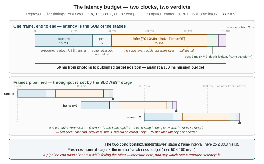
The numbers are representative rather than universal — the whole point of the next section is that they must be measured, not copied — but their shape is typical and instructive. Inference, the stage every optimization guide obsesses over, is half the bill. Capture is a heavy line item that no model compression touches: the sensor must expose (longer in low light — a robustness thread picked up later), read out, and push 921,600 bytes over USB before software sees anything. Preprocessing is the resize-letterbox-normalize gauntlet of the Images as Data chapter, cheap but not free. Postprocessing covers non-maximum suppression, the depth lookup, and the pixel-to-vehicle-frame transform that turns a box into the target position. Summed: 50 ms of age on every published position — within the 100 ms budget, with room for the degradation that field conditions will impose.
The pipelined view yields the throughput verdict. With stages overlapped, a new result emerges once per slowest stage — 25 ms here, a 40 FPS ceiling — so the camera’s 30 FPS is sustained with headroom. But the same figure shows how quickly the ledger can flip: swap in a model whose inference takes 40 ms, and the bottleneck stage exceeds the 33.3 ms frame interval; the pipeline now completes at most 25 frames per second, frames drop, and — if the queueing discipline is wrong — latency compounds frame over frame. One stage’s overrun degrades both conditions at once, which is why the budget is kept as a table of stages and re-measured whenever any stage changes. The habit should feel familiar: it is Part I’s power budget and the TinyML chapter’s memory bill, transposed into milliseconds.
16.5 Measuring Honestly
The latency budget is only as good as its numbers, and timing a neural network is strewn with ways to get flattering, wrong ones. Four disciplines separate a measurement from an anecdote.
Exclude warm-up. The first inference after a model loads pays one-time costs — kernel compilation, memory allocation, cache population — that can run to hundreds of milliseconds and will never recur in flight. A benchmark that includes them overstates latency; a benchmark of only the first few frames can also understate steady-state FPS while the GPU’s clocks ramp. Run tens of inferences before recording anything.
Report the tail, not just the mean. Latency is a distribution, and control deadlines are violated by its worst cases, not its average. A pipeline averaging 30 ms with a 99th-percentile of 80 ms misses a 60 ms deadline about once every hundred frames — at 30 FPS, several times every ten seconds, each miss a stale position published to the steering loop. The mean hides this entirely; the percentiles are the honest summary, and the maximum over a long run is worth recording besides.
Run long enough to get hot. An embedded computer under sustained inference load heats up, and when it reaches its thermal limit it protects itself by cutting clock speeds — thermal throttling — at which point latency quietly rises. The effect takes minutes to appear and a 30-second benchmark will never see it, which is exactly why it surfaces in the field instead: the mission’s twentieth minute, a warm afternoon, a heatsink sized for the bench. Benchmarks intended to clear a flight readiness bar run for the duration of a flight, and log temperature alongside latency so the correlation is visible.
Measure on the target, under the mission’s load. The Jetson’s GPU shares memory bandwidth, power budget, and (for some stages) CPU cores with everything else Part II put on the aircraft — the ROS 2 graph, the MAVLink bridge, logging, the camera driver itself. A model benchmarked alone on the bench inherits resources the mission will take back. The previous chapter’s doctrine — the model is a component, not the system — becomes a measurement rule here: the number that matters is the latency of the assembled stack, measured at the output topic, while everything else runs.
The measurement itself needs no framework, only care with what is timed:
import time
import numpy as np

lat = []
for i in range(1000):
    frame = get_latest_frame()          # drops stale frames; returns newest
    t0 = time.perf_counter()
    boxes = detector.infer(frame)       # preprocess + model + NMS inside
    lat.append((time.perf_counter() - t0) * 1000.0)

lat = np.array(lat[50:])                # discard warm-up
print(f"mean {lat.mean():.1f} ms   p50 {np.percentile(lat, 50):.1f}"
      f"   p99 {np.percentile(lat, 99):.1f}   max {lat.max():.1f}")
Note what this loop measures and what it does not: it times preprocess-through-postprocess — the software stages — but starts its clock after capture, so the capture line of the latency budget must be measured separately (typically from the frame’s hardware timestamp, which the camera driver attaches, to the moment get_latest_frame returns). Timing from the hardware timestamp to the published topic, inside the running ROS 2 graph, is the full end-to-end figure; the snippet’s figure is the part the model choice controls. Keeping the two straight — and saying which one a reported “latency” is — is half of measurement honesty.
16.6 The Accuracy–Speed Frontier
Suppose the measurement disappoints: the tail latency blows the budget, or the sustained FPS sags under load. Two of the levers are inherited from earlier chapters and need only naming: quantization (the TinyML chapter’s factor of two-to-four, already spent if the deployment followed that chapter) and input resolution (the Images as Data chapter’s quadratic lever, pulled against pixels-on-target and detection range). The third lever is the one this Part has so far held fixed: the model itself. Modern detector families are published as a ladder of sizes — the same architecture scaled in depth and width — and the YOLOv8 family the pipeline trains is typical: nano, small, medium, large, extra-large, from 3.2 million parameters to 68.2 million. The published benchmarks of the family, plotted in Figure 16.2, form the curve on which every model-size decision is made.
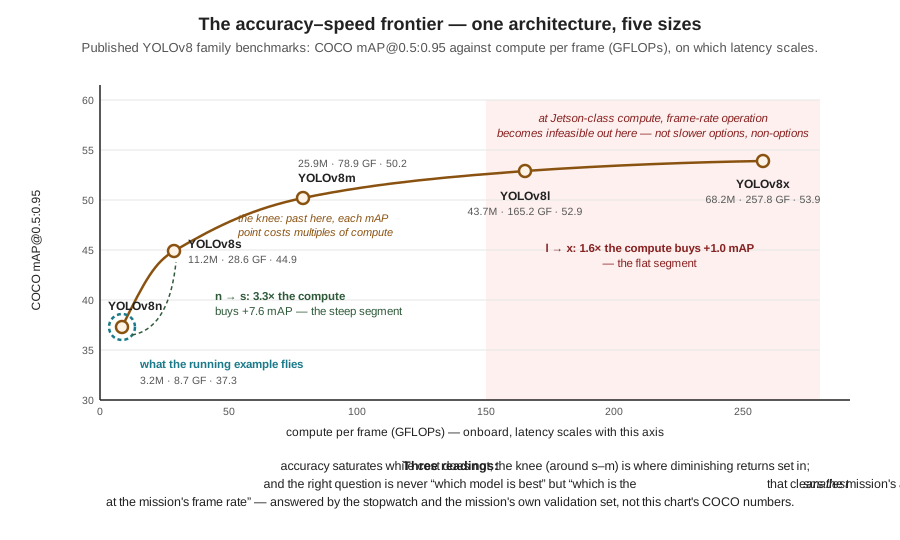
Three readings of the curve matter more than any point on it. First, its shape: accuracy saturates while cost does not. The step from nano to small buys 7.6 points of COCO mAP for 3.3× the compute — a defensible trade; the step from large to extra-large buys 1.0 point for 1.6× the compute on top of an already-unflyable base. The saturation is not an accident of this family but the general pattern of scaling within a task: the easy accuracy is bought first, cheaply, and each further point costs more than the last. Second, the latency axis is the binding one onboard: on the companion computer’s fixed compute budget, a model’s GFLOPs translate roughly into its inference time, and somewhere along the curve — the shaded region of the figure — the frame-rate condition of the first section fails outright, making the upper family members not slower options but non-options. Third, and most important, the question the curve answers: not “which model is best” — the top of the curve is best, uselessly — but “which is the smallest model that clears the mission’s accuracy floor at the mission’s frame rate.” That is the same question the TinyML chapter’s placement problem asked of hardware tiers, now asked within a tier, and it explains the deployment folklore the source material compresses into a tip: start with the nano model and scale up only when measurement says the accuracy floor is unmet. Starting large and shrinking under schedule pressure runs the same search from the expensive end.
Two refinements keep the frontier honest in practice. The published mAP figures are COCO numbers — eighty everyday object classes — and a two-class goose detector fine-tuned per the previous chapter will not match them numerically; the ordering and the shape transfer, the absolute values do not, so the family comparison worth trusting is run on the mission’s own validation set. And the frontier interacts with the resolution lever: a larger model at a smaller input can land at the same latency as a smaller model at full input with different accuracy — the small model preserving small-object range (more pixels on the distant goose), the large one classifying what it sees more reliably. The two-lever grid — family member × input size — is small enough to measure exhaustively in an afternoon of benchmarking, and for a mission whose targets are 7-pixel smudges at range, the pixels usually win. There is no closed-form answer here, which is the section’s real lesson: the frontier tells the engineer where to look; only the stopwatch and the validation set say where to land. The “best” model, as the source material puts it, is a system-level trade-off — accuracy, latency, energy, memory, robustness, and the cost of being wrong, negotiated together.
16.7 From Frames to Decisions: Tracking
Everything so far treats each frame as an isolated question. But the mission does not consume frames — it consumes decisions: begin the deterrence run, steer toward this goose, break off. And between per-frame detections and sound decisions sits a gap that latency and accuracy numbers do not describe. A detector operating deliberately down-threshold — as the previous chapter argued the running example should, trading precision for recall — emits occasional false positives by design; even on true geese, boxes flicker as confidence hovers near threshold, vanish for a frame of motion blur, and reappear. A state machine wired directly to raw detections inherits every flicker: it would launch a deterrence run at a shadow, abort when a real goose blinks out for two frames, and re-acquire the same bird as a new target ten times a minute. The missing machinery is object tracking: associating detections across frames so that the same physical goose keeps the same identity over time, converting a stream of stateless boxes into a set of object histories. Figure 16.3 shows the transformation on a strip of frames.
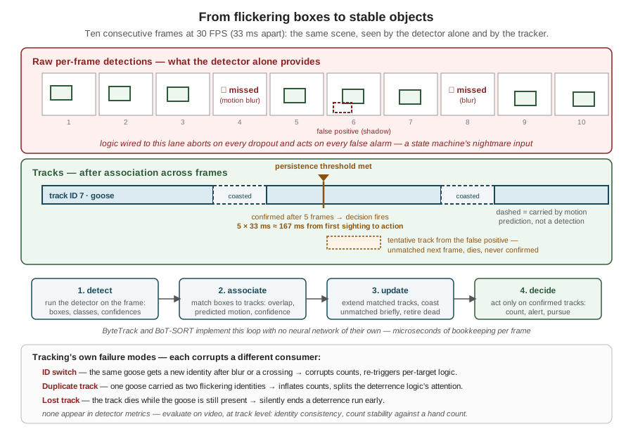
The mechanics are lighter than the word “tracking” suggests. Each frame, the tracker matches the detector’s new boxes against its live tracks using cheap evidence — box overlap with the track’s last position, a constant-velocity prediction of where the track should be now, detection confidence — then extends matched tracks, lets unmatched tracks coast on their predicted motion for a few frames before retiring them, and opens tentative tracks for unmatched detections. Standard lightweight implementations such as ByteTrack and BoT-SORT do exactly this with no neural network of their own and no training: their cost is microseconds of bookkeeping per frame, which is why the tracking line of the latency budget was near-zero. For that price the mission logic gains three things it cannot get from any single frame: stability (one goose is one object, not a re-detected stranger every frame), motion (a track has a velocity — where the goose is heading, which the deterrence approach can lead), and evidence accumulation — the ability to require that an object persist before acting on it.
That last item is where tracking rejoins this chapter’s subject, because persistence is bought with time. A persistence threshold of \(N\) consecutive frames means a track is confirmed — and the deterrence decision fires — only after the object has survived \(N\) association rounds, which at frame interval \(\Delta t\) adds a decision delay of \(N \Delta t\): five frames at 30 FPS is 167 ms between first genuine sighting and action. That delay is not overhead to be minimized to zero; it is the price of not chasing shadows, and it is tuned, like the confidence threshold it complements, in mission currency. A spurious deterrence run costs a full flight leg of battery; 167 ms of deliberation costs 80 cm of goose travel. The running example takes that trade — and takes the symmetric one on the way out, coasting a confirmed track through several missed frames before declaring the goose gone, so one blurred frame does not abort a deterrence run in progress. Both thresholds lengthen the effective latency between the world changing and the system’s model of it changing; both are the reason the raw pipeline latency needed headroom under its 100 ms budget rather than merely meeting it.
Tracking earns its keep, and then it fails in its own ways, worth naming because each corrupts a different downstream consumer. An ID switch — the same goose re-identified as a new object after a blur or a crossing with another bird — corrupts counting and re-triggers per-target logic. A duplicate track — one goose carried as two flickering identities — inflates counts and can split the deterrence logic’s attention. A lost track — the track dying while the goose remains — silently ends a deterrence run early. None of these appear in detector metrics; they are evaluated on video with track-level checks — identity consistency, count stability over a sequence with known ground truth — one more instance of this chapter’s refrain that the deployed system must be measured at the level its consumers consume.
16.8 Robustness: When the World Leaves the Dataset
The previous chapter’s split discipline produced an honest validation score — honest, that is, about footage statistically like the dataset. The field makes no such promise. A deployed model’s inputs drift away from its training distribution — the phenomenon called distribution shift — and when they do, the validation score stops predicting anything without announcing that it has stopped: the model still runs, still emits confident boxes, and is simply wrong more often. A drone is close to the worst platform imaginable on this axis. Its viewpoint changes continuously with altitude and attitude; its scenes change with weather, season, and site; its own propulsion vibrates the camera; and its mistakes cost energy and, in the limit, safety. The maxim from the source material deserves its italics: a model that works in a notebook is not necessarily ready to fly. Figure 16.4 catalogs the three failure modes a flying camera meets first, with the symptom each produces and the mitigations each admits.
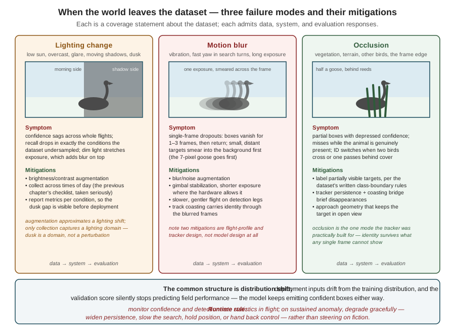
The three columns share a structure worth extracting. Each failure mode is, at bottom, a coverage statement about the dataset — the conditions under which the detector degrades are precisely the conditions the training distribution undersampled — which is why the first mitigation in every column is data: targeted augmentation for the perturbation’s cheap approximations, targeted collection for the real thing. The distinction between those two matters and the source material states it exactly: augmentation simulates small variations around known examples — a brightness shift, a synthetic blur — and cannot conjure missing domains; no augmentation of daytime meadow footage produces the statistics of dusk, rain, or a new site. Augmentation stretches coverage; only collection extends it. This is the closing loop of the previous chapter wearing its field clothes: failures cluster by condition, and the cluster names the next collection flight. The second mitigation in every column is system design rather than model design — stabilization hardware, flight profiles that respect the camera (slower, smoother legs while detecting), tracker persistence carrying identity through transient dropouts — a reminder that the perception system extends well beyond the network. And the third is evaluation design: reporting metrics per condition (morning versus noon, calm versus windy, near versus far) rather than as one pooled number, so that a model strong on average and blind at dusk cannot hide inside its own mean. The habit of building that per-condition table before collecting data — deciding what the mission envelope contains and measuring coverage against it — is the cheapest robustness tool in the kit.
One mitigation belongs to no column because it belongs to all of them: admitting, at runtime, that the model may currently be wrong. A perception system cannot detect its own distribution shift directly, but it can watch proxies — detection confidence trending down, detection rate collapsing or spiking, track churn rising, inputs statistically unlike anything calibrated for — and treat sustained anomaly as a signal to degrade gracefully: widen persistence thresholds, slow the search, hold position, or hand the decision back to the operator, rather than continue steering on fiction. Part II built exactly this reflex into the flight stack — the watchdog, the failsafe ladder, the principle that every autonomous behavior needs a defined behavior for its own failure — and the perception system, as the newest autonomous behavior aboard, owes the same contract. The Detector node that publishes target positions should also publish its own health, and the state machine that consumes the first should consume the second.
16.9 A Note on Responsibility
There is a last trade-off in this chapter’s territory that is not measured in milliseconds. The system now assembled — a camera, a detector, a tracker, an aircraft that acts on what they say — watches a physical place continuously, and its errors move a machine through that place. That raises obligations beyond engineering correctness. On-device inference, adopted in Part I for bandwidth and here for latency, turns out to carry a privacy dividend — raw imagery of whoever walks through the protected area never leaves the aircraft, and the system can be designed to transmit and retain only derived summaries — but the dividend is not automatic and it is not absolution: what is stored, for how long, who may access it, and what the system does about people it was never meant to watch are design decisions, made explicitly or made badly. Dataset bias has already appeared in this Part as an accuracy problem; it returns as a fairness and safety problem when the failures cluster on particular conditions, places, or bystanders. And a wildlife-deterrence system in particular owes an account of its effects on the animals themselves. These questions get a chapter of their own — The Ethics and Ecology of Autonomous Wildlife Management, in Part V — with the full treatment of privacy-by-design, bias auditing, and the ecology of deterrence. They are flagged here, before the system flies, for one reason: responsible AI is a set of design requirements, and design requirements bind earliest, when the logging format, the retention policy, and the evaluation table are still cheap to change.
The Part’s arc is now complete: pixels became tensors, tensors met budgets, budgets shaped a trained detector, and this chapter held the assembled pipeline to the two clocks the mission runs on — then smoothed its output into objects worth acting on and armored it against the field. What the running example’s perception stack now publishes is exactly what Part II’s state machine was built waiting for: a confirmed, tracked, health-annotated target position, fresh to within a measured bound. One chapter remains before Part IV takes up the autonomy that decides what to do with that position: a case study that holds this Part’s entire approach against the published record of detecting animals from the air — and against the measured behavior of the geese themselves.
16.10 Check Your Understanding
- A vendor demo shows a detection overlay updating smoothly at 30 FPS, and the vendor claims the system is “real-time.” State the two separate conditions a real-time perception pipeline must satisfy, and describe a stage structure under which this demo passes one condition while carrying 150 ms of end-to-end latency. Which condition does the smooth overlay actually demonstrate?
The conditions are throughput — sustained FPS at least the rate at which the mission needs fresh answers (bounded by the slowest pipeline stage) — and freshness: end-to-end latency (the sum of all stages) within the mission’s staleness budget. A five-stage pipeline whose stages each take 30 ms, run concurrently, emits a new result every 30 ms (33 FPS — smooth overlay) while each result is 150 ms old on arrival. The overlay demonstrates only throughput: it shows how often a new answer appears, not how old each answer is. For a display, age barely matters; for a loop steering toward a moving animal, 150 ms is 75 cm of goose travel at 5 m/s, and the latency condition must be verified separately, by measuring from the frame’s hardware timestamp to the published output.
- A pipeline’s measured stages are: capture 15 ms, preprocess 5 ms, inference 40 ms, postprocess 3 ms, track-and-publish 2 ms, with a 30 FPS camera (33.3 ms frame interval). Compute the end-to-end latency and the sustained throughput ceiling, state which real-time condition fails, and explain what happens to latency over time if the pipeline naively queues every frame instead of dropping stale ones.
Latency is the sum: \(15 + 5 + 40 + 3 + 2 = 65\) ms. Throughput is set by the slowest stage: one result per 40 ms, a ceiling of 25 FPS. The freshness condition can still pass (65 ms is under a 100 ms budget), but the throughput condition fails: 25 FPS cannot keep up with 30 FPS arrival. With naive queueing, frames arrive every 33.3 ms and leave every 40 ms, so the queue grows by one frame every ~200 ms and the age of the frame being processed grows without bound — after a minute the detector is analyzing footage from seconds ago, and the published positions are systematically stale even though each individual frame still takes only 65 ms of processing. Dropping stale frames caps latency at the pipeline depth but concedes that only ~25 of every 30 frames are seen; fixing the condition properly requires shrinking the 40 ms bottleneck stage (smaller model, lower resolution) or accepting a lower target rate.
- Using the published YOLOv8 family figures (n: 8.7 GFLOPs / 37.3 mAP; s: 28.6 / 44.9; m: 78.9 / 50.2; l: 165.2 / 52.9; x: 257.8 / 53.9), compute the compute-cost multiplier and the mAP gain for the steps n→s and l→x, and state the general shape of the frontier these two numbers illustrate. Then explain why the absolute mAP values should not drive the running example’s model choice, and what should.
n→s: \(28.6/8.7 \approx 3.3\times\) the compute for \(44.9 - 37.3 = 7.6\) mAP. l→x: \(257.8/165.2 \approx 1.6\times\) the compute for \(53.9 - 52.9 = 1.0\) mAP. The frontier rises steeply at the small end and flattens at the large end — accuracy saturates while cost does not, so each further point of accuracy costs more than the last. The absolute values are COCO benchmarks: eighty everyday classes, a distribution unlike a two-class aerial goose task, so a fine-tuned goose detector’s numbers will differ; only the ordering and shape transfer. The choice should be driven by measurements on the mission’s own validation set and hardware: the smallest family member whose measured accuracy clears the mission’s floor at the mission’s frame rate — starting from nano and scaling up on evidence, not down from the top under schedule pressure.
- A detector benchmarks at a mean latency of 28 ms over a 30-second bench test, and the team declares a 60 ms deadline comfortably met. Give two distinct reasons this conclusion can be wrong in flight even if the measurement was performed correctly as far as it went, and state the benchmarking discipline that catches each.
First, the mean hides the tail: a distribution with mean 28 ms can carry a 99th percentile above 60 ms, and at 30 FPS a 1-in-100 violation recurs several times every ten seconds, each one a stale position published to the control loop. Discipline: report percentiles (p95/p99) and the maximum, not the mean alone. Second, 30 seconds is too short and too idle: thermal throttling appears minutes into sustained load — the processor cuts clocks as it heats, raising latency — and a bench test without the mission’s competing processes (ROS 2 graph, logging, camera driver, MAVLink bridge) lends the model memory bandwidth and cores the mission will reclaim. Discipline: benchmark for a flight’s duration, on the target, with the full stack running, logging temperature alongside latency. (Warm-up is the symmetric error in the other direction — including the first inferences’ one-time costs overstates latency — excluded by discarding initial iterations.)
- The running example’s tracker requires 5 consecutive frames of persistence at 30 FPS before confirming a track, and coasts a confirmed track for up to 4 missed frames before retiring it. Compute the decision delay on first sighting and the maximum blindness the coasting rule tolerates, and explain — in mission currency — what each threshold purchases and what raising each further would cost.
Confirmation delay: \(5 \times 33.3 \approx 167\) ms between first genuine detection and the deterrence decision — during which a goose at 5 m/s moves about 80 cm. Coasting: \(4 \times 33.3 \approx 133\) ms of continuous dropout tolerated before a confirmed track dies. Confirmation purchases immunity to acting on single-frame false positives — a spurious deterrence run costs a flight leg of battery, far more than 167 ms of deliberation. Coasting purchases immunity to aborting a deterrence run over one or two blurred frames — a lost track mid-run silently ends the mission’s core behavior. Raising the confirmation threshold further delays every legitimate response (and a fast-moving goose may exit the frame before confirmation); raising the coasting window further means steering longer on a motion prediction rather than a measurement — the track can drift arbitrarily far from the real animal, and a genuinely departed goose keeps consuming deterrence effort.
- During an evening flight, the detector’s confidence scores sag across the whole flight and recall drops sharply, though the model performed well on the validation set. A teammate proposes fixing it by adding synthetic brightness reduction to the training augmentation. Diagnose the failure mode, evaluate the proposal — including what augmentation can and cannot fix — and name the runtime behavior the system should have exhibited in the meantime.
This is distribution shift, lighting-change column: dusk imagery is statistically unlike the (presumably daytime) training and validation distribution, so the validation score stopped predicting field performance — and did so silently. Brightness augmentation is a partial, legitimate first step: it simulates small photometric variations around known examples and can recover some robustness cheaply. But dusk is closer to a missing domain than a perturbation — changed color balance, longer exposures adding motion blur, different backgrounds and animal behavior — and augmentation cannot conjure a domain the dataset lacks; the durable fix is targeted collection of evening footage (with the per-condition evaluation table extended to report dusk performance separately, so the gap is visible rather than pooled into a mean). At runtime, the sustained confidence anomaly should have triggered graceful degradation — widened persistence thresholds, a slowed search, holding position, or handing back to the operator — because a perception system that cannot notice its own degradation steers the vehicle on fiction.
16.11 Try It
Part 1 — build the latency budget, then break it. Take the detector you trained in the previous chapter’s exercise (any YOLOv8n fine-tune serves) and benchmark it honestly on the most constrained hardware you have: time 1,000 inferences with time.perf_counter, discard the first 50, and report mean, p50, p99, and max. Then extend the measurement outward into a full budget: time preprocessing separately, time capture by comparing frame timestamps against arrival times if your camera exposes them, and lay out your own version of Figure 16.1. Now stress it: run the benchmark again for ten sustained minutes while logging latency per 10-second window (and processor temperature, if exposed) and look for the throttling drift; then run it once more with a competing CPU load (a video encode, a compile) and quantify what contention costs your p99. Finally, sweep the two levers: benchmark the n and s family members at input sizes 640, 416, and 320 — a 3 × 2 grid — and plot your own accuracy-latency frontier from the grid’s validation mAP and measured p99, marking which cells meet a 30 FPS throughput condition on your hardware. Write one sentence naming the cell you would fly and the two numbers that justify it.
Part 2 — add a tracker and measure what it buys. Run your detector over two or three minutes of continuous video containing your target class and log raw per-frame detections. First quantify the flicker: count single-frame false positives and 1–3-frame dropouts of genuinely present objects — the noise a state machine wired to raw detections would inherit. Then add tracking: either integrate a standard lightweight tracker (ByteTrack via the Ultralytics model.track() interface is a one-line change) or implement the chapter’s loop yourself — associate by IoU against a constant-velocity prediction, confirm after \(N\) frames, coast for \(M\). Measure the transformation: how many false positives survive to confirmed tracks at \(N = 5\); how many dropouts are bridged by coasting at \(M = 4\); how the object count over the clip compares, raw versus tracked, against a hand count. Then find the failure modes: engineer an occlusion (two targets crossing, or one passing behind cover) and observe whether you get an ID switch or a lost track, and at what coasting window the track survives. Close by computing your decision delay \(N \Delta t\) and writing two sentences: one defending your \(N\) and \(M\) in mission currency, one stating which tracking failure mode your consumer — count, alert, or pursuit — is most sensitive to, and why.
Related Lab: See Appendix B for the lab assignment that applies this chapter’s concepts.