9 Closed-Loop Control: PID Theory for Multirotors
Part I closed with a finished vehicle and a promise: the hardware will not change again, and everything from here forward is software running on the two computers it carries. This chapter starts where that promise pointed — at the innermost of the three nested loops the previous chapter identified, the one running on the flight controller at kilohertz rates, the one whose deadline cannot be missed. The Putting It Together chapter could say only that the flight controller “resolves the error between commanded and actual attitude into four motor commands.” This chapter is about how. The mechanism is feedback control, its workhorse is the proportional–integral–derivative (PID) controller, and by the end the sentence in quotes will have become an equation, a worked numeric design, a dozen lines of code, and a set of symptoms you can diagnose from the way an aircraft misbehaves.
The material earns its place at the front of Part II for a blunt reason: nothing above it works if it doesn’t. Every mission script, every offboard setpoint, every clever behavior the rest of this book builds ends its life as a request handed to these loops, and the request is granted only as well as the loops are tuned. A vehicle whose rate controller oscillates cannot hold a camera steady enough for the perception of Part III; one whose altitude controller carries a steady-state error will fly its search grid at the wrong height. Control is the floor everything else stands on.
9.1 Learning Objectives
- Explain why a multirotor is unflyable without feedback: the plant is underactuated, its hover is an unstable equilibrium, and it is continuously disturbed.
- Derive the PID control law \(u(t) = K_p e(t) + K_i \int_0^t e(\tau)\,d\tau + K_d \frac{de(t)}{dt}\) from the three questions a controller can ask of its error signal, and state each term’s physical effect on a multirotor’s response.
- Design a PD altitude-hold controller for a vehicle of known mass by choosing a natural frequency and damping ratio, and verify the design against the aircraft’s thrust margin.
- Identify overshoot, oscillation, sluggishness, and steady-state error as tuning symptoms, attribute each to a specific gain, and state the standard remedy.
- Convert the continuous PID law into the sampled-data form that actually runs on a flight controller, including integrator clamping and derivative filtering, and explain why each modification exists.
- Explain why multirotor flight control uses a cascade of loops — position, velocity, attitude, angular rate — rather than one PID, and why the innermost rate loop is tuned first.
9.2 Key Vocabulary
- Setpoint — the reference value \(r(t)\) a control loop is asked to achieve: a commanded altitude, attitude, or angular rate. In a cascaded controller, each loop’s output is the next inner loop’s setpoint.
- Plant — the physical system a controller acts on. Here, the quadrotor’s rigid-body dynamics: four motor thrusts in, translational and rotational motion out.
- Proportional gain (\(K_p\)) — the weight on the present error. It acts like a spring stiffness: the command it produces is proportional to how far the vehicle currently is from the setpoint.
- Integral gain (\(K_i\)) — the weight on the accumulated error. It builds up a corrective command as long as any error persists, which is what removes steady offsets caused by unmodeled forces such as a payload shift or a weak motor.
- Derivative gain (\(K_d\)) — the weight on the error’s rate of change. It acts like a damper, opposing rapid motion toward or away from the setpoint, which is what suppresses overshoot.
- Steady-state error — the offset that remains after the transient response has died out. A proportional-only controller facing a constant disturbance always leaves one, because it needs a nonzero error to produce a nonzero command.
- Overshoot — the amount by which the response passes beyond the setpoint before settling back, a symptom of too little damping relative to stiffness.
- Cascaded control loop — an architecture in which a slow outer controller does not command the actuators directly but instead generates the setpoint for a faster inner controller, repeated over as many layers as the plant’s time scales demand.
- Integrator windup — the failure mode in which the integral term keeps accumulating while the actuators are saturated and cannot act on it, then discharges as a large overshoot once the vehicle finally catches up; prevented by clamping the integrator.
9.3 Why a Multirotor Cannot Fly Open Loop
An open-loop controller computes its command from the request alone: to climb one metre, add some thrust for some duration, and hope. For a few plants — a stepper motor, a toaster — hoping works, because the plant is stable and the disturbances are small. A multirotor fails every part of that description, for three reasons the vehicle of Part I makes concrete.
First, the plant is underactuated. The aircraft has six degrees of freedom — position \(x, y, z\) and attitude roll \(\phi\), pitch \(\theta\), yaw \(\psi\) — but only four independent inputs, the four motor thrusts. It cannot accelerate sideways while staying level; as the Anatomy of a Multirotor chapter established, translation is bought with tilt, and yaw is bought with the drag-torque imbalance between the two counter-rotating propeller pairs. Rotation and translation are permanently coupled, so any position command is really an attitude command in disguise.
Second, hover is an unstable equilibrium. All four thrusts summing exactly to weight, with the thrust vector exactly vertical, is a balance point — but nothing restores it. Tilt the aircraft a degree and the thrust vector tilts with it, producing a sideways acceleration that grows the disturbance rather than fighting it. A fixed-wing aircraft can be built with passive aerodynamic stability; a multirotor has none. The often-quoted consequence from the previous chapter — that a stall of a tenth of a second in the attitude loop is the end of the flight — is just this instability stated as a deadline.
Third, the plant is continuously disturbed. Wind gusts apply torques; the battery sags, changing thrust per unit command as the flight proceeds; motors and propellers are never perfectly matched; a payload sits a centimetre off the centre of gravity. None of these appear in any feedforward calculation, and all of them push the state away from wherever it was commanded to be.
The remedy is to stop computing commands from the request and start computing them from the error. A closed-loop controller continuously compares the setpoint \(r(t)\) against the measured (in practice, estimated) output \(y(t)\) and forms
\[e(t) = r(t) - y(t),\]
the tracking error, which is the only signal the controller ever consumes. Figure 9.1 shows the structure. The loop answers three questions, over and over, at whatever rate the plant demands: where am I, where should I be, and what command shrinks the difference?
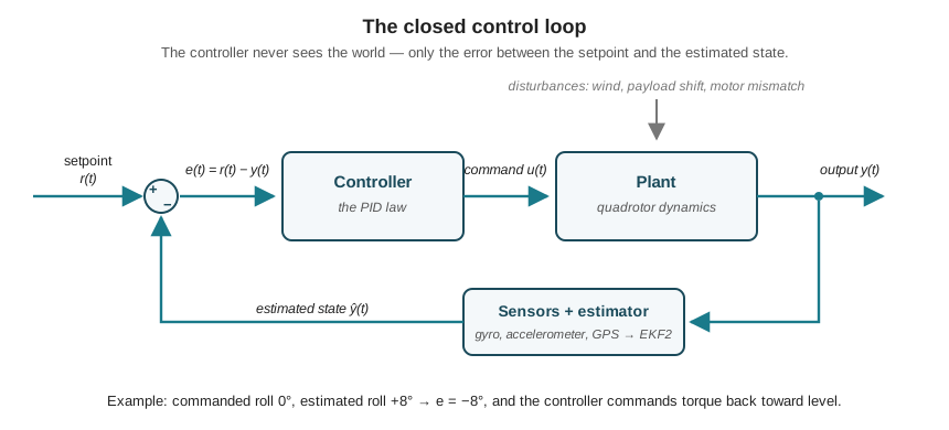
Two details in the figure deserve emphasis because they recur all book long. The feedback path runs through sensors and an estimator, not through the world directly: as the Sensing the World chapter showed, the controller acts on EKF2’s fused estimate \(\hat{y}(t)\), with all the bias-tracking and outlier rejection that implies, and a controller is only ever as honest as the estimate it is fed. And the sign convention matters: with \(e = r - y\), a vehicle rolled to \(+8^\circ\) against a commanded \(0^\circ\) produces \(e_\phi = -8^\circ\), and the controller output — a negative roll torque — is what rotates it back toward level. Every loop in this chapter, and every loop in the PX4 firmware, is built around exactly this signal.
9.4 The PID Control Law
Given the error signal, what command should the controller produce? The PID answer is that there are exactly three useful questions to ask of \(e(t)\) — what is it now, what has it been, and where is it going — and that the command should be a weighted sum of the three answers:
\[u(t) = K_p\, e(t) \;+\; K_i \int_0^t e(\tau)\, d\tau \;+\; K_d\, \frac{de(t)}{dt}.\]
The three gains \(K_p\), \(K_i\), \(K_d\) are the entire design space, and each maps onto a distinct physical behavior of the aircraft.
The proportional term is stiffness. It responds to the present error, immediately and in proportion: a large tilt produces a large corrective torque, a small tilt a small one. A vehicle with low \(K_p\) feels soft and sluggish, leaning downwind like a reed and returning lazily. Raise \(K_p\) and it stiffens — corrections come faster and harder. Raise it too far and the vehicle overshoots the setpoint, corrects back, overshoots again, and oscillates: the command is always proportional to an error that the vehicle’s inertia has already carried it past.
The integral term is memory. A proportional controller has a structural blind spot: it can only produce a command while there is an error, so any constant disturbance settles into a standoff — a permanent offset at which the proportional command exactly balances the disturbance and nothing changes. Suppose one motor is a few percent weak, or the battery of the running example sits a centimetre aft of the vehicle’s centreline. The aircraft hovers with a small persistent tilt, and \(K_p\) alone will hold that tilt forever. The integral term accumulates the error over time, growing its contribution until the bias is cancelled and the error is actually zero. Its cost is sluggishness of a particular kind: too much \(K_i\) produces slow, wallowing oscillation, and — as the next sections make precise — an integrator that accumulates while the motors are saturated causes the overshoot called windup.
The derivative term is damping. It responds not to the error but to its trend. If the vehicle is rotating rapidly toward the setpoint, the derivative term begins braking before the setpoint is reached, exactly as a damper resists velocity regardless of position. This is what converts an oscillatory response into a crisply settling one. Its cost is noise sensitivity: differentiation amplifies exactly the high-frequency content — gyro noise, propeller vibration at the blade-passage frequencies the Materials and Power chapter computed — that the rest of the system works to suppress. Too much \(K_d\) shows up as a hot, twitchy vehicle whose motors buzz in response to vibration the pilot cannot even see.
The three terms are not independent knobs so much as three forces in negotiation — stiffness pulling toward the setpoint, damping resisting the speed of the pull, memory removing whatever offset the other two leave behind. Tuning is the act of setting the terms of that negotiation, and it becomes concrete the moment real numbers are attached.
9.5 A Worked Design: Altitude Hold
Take the running example’s aircraft as Part I left it: all-up mass \(m = 2.2\) kg, maximum static thrust about \(4.0\) kgf \(= 39.2\) N, hover thrust \(mg = 2.2 \times 9.81 = 21.6\) N, leaving a climb margin of about \(17.7\) N above hover. The task is the simplest loop on the vehicle: hold a commanded altitude \(z_d\).
Near hover, write total thrust as hover thrust plus a correction, \(T = mg + \Delta T\). Newton’s second law for the vertical axis, neglecting drag at the low vertical speeds of altitude hold, is
\[m\ddot{z} = T - mg = \Delta T.\]
Let the controller be PD for now — proportional and derivative, with the integral term’s role examined afterward — commanding
\[\Delta T = K_p\, e - K_d\, \dot{z}, \qquad e = z_d - z.\]
(Using \(-\dot z\) rather than \(\dot e\) is the standard derivative-on-measurement form; for a constant setpoint they are identical, and for a setpoint that jumps it avoids differentiating the jump.) Substituting into the dynamics and using \(\ddot z = -\ddot e\), \(\dot z = -\dot e\) for constant \(z_d\) gives a second-order linear system in the error:
\[ \begin{aligned} m\ddot{e} + K_d\, \dot{e} + K_p\, e &= 0,\\ \text{i.e.}\quad \ddot{e} + \frac{K_d}{m}\,\dot{e} + \frac{K_p}{m}\, e &= 0. \end{aligned} \]
Comparing against the canonical form \(\ddot e + 2\zeta\omega_n \dot e + \omega_n^2 e = 0\) identifies the two quantities a designer actually chooses: the natural frequency \(\omega_n = \sqrt{K_p/m}\), which sets how fast the loop responds, and the damping ratio \(\zeta = K_d / (2 m \omega_n)\), which sets how the response settles. This is the central trick of classical design — pick the behavior, then read off the gains:
\[ \begin{aligned} K_p &= m\,\omega_n^2,\\ K_d &= 2\,\zeta\,\omega_n\, m. \end{aligned} \]
Choose a response with a time constant under a second and essentially no overshoot: \(\omega_n = 2.0\) rad/s and \(\zeta = 0.9\). Then
\[ \begin{aligned} K_p &= m\,\omega_n^2 = 2.2 \times (2.0)^2 = 8.8\ \text{N/m},\\ K_d &= 2\,\zeta\,\omega_n\, m = 2 (0.9)(2.0)(2.2) = 7.92\ \text{N}\cdot\text{s/m}. \end{aligned} \]
Two checks make this a design rather than an arithmetic exercise. Overshoot: for a second-order system the peak overshoot is \(M_p = \exp\!\left(-\pi\zeta/\sqrt{1-\zeta^2}\right)\), and at \(\zeta = 0.9\) that is \(\exp(-2.827/0.436) \approx 0.0015\) — about 0.15 %, invisible in flight. Saturation: a 1 m altitude error commands \(8.8\) N of extra thrust against the \(17.7\) N available, comfortable; a 2 m error commands \(17.6\) N and sits at the very edge of the climb margin. Larger steps saturate the motors, and the linear analysis above stops describing the vehicle — a fact that will matter shortly.
Now break the design deliberately, because the failure modes are the point. Figure 9.2 shows all three responses to the same 1.0 m climb command.
Too much proportional gain. Multiply \(K_p\) by ten, to 88 N/m, leaving \(K_d\) alone. The closed-loop parameters follow from the same two formulas, run backward:
\[ \begin{aligned} \omega_n &= \sqrt{K_p/m} = \sqrt{88/2.2} = \sqrt{40} = 6.32\ \text{rad/s},\\ \zeta &= \frac{K_d}{2 m \omega_n} = \frac{7.92}{2(2.2)(6.32)} = 0.285,\\ M_p &= \exp\!\left(\frac{-\pi (0.285)}{\sqrt{1-0.285^2}}\right) = \exp(-0.93) \approx 0.39. \end{aligned} \]
The response is fast — and rings, overshooting the setpoint by 39 % and oscillating through several diminishing cycles. This is the universal signature of excessive gain, and the standard remedy is exactly what the algebra says it is: reduce \(K_p\), or restore the balance by adding derivative damping until \(\zeta\) is back near critical. Worse, the linear prediction is optimistic here: a 1 m error now commands 88 N of correction against 17.7 N of authority, so the motors saturate hard and the real response is uglier than the formula admits. On an attitude loop the same mistake is more than ugly — a 39 % overshoot in roll near the ground, or near the 122 m ceiling the Airspace Law chapter established, is an incident.
No integral term. Suppose the vehicle carries 200 g the controller’s model does not know about — mud on the airframe, a heavier battery, the payload creep every field program experiences. The feedforward hover term \(mg\) is now short by \(0.2 \times 9.81 = 1.96\) N, a constant downward disturbance. The PD loop settles where proportional command balances deficit: \(K_p e_{ss} = 1.96\) N, so
\[e_{ss} = \frac{1.96}{8.8} = 0.22\ \text{m}.\]
The aircraft flies its entire mission 22 cm below every altitude it is asked for — stable, smooth, and wrong. This is steady-state error, and no amount of \(K_p\) or \(K_d\) tuning removes it; raising \(K_p\) only shrinks it at the price of the ringing computed above. The integral term is the cure. With an integral gain \(K_i = 2\) N/(m·s), the integrator accumulates at \(K_i e \approx 0.45\) N/s while the error stands at 0.22 m, so it would need roughly \(1.96/0.45 \approx 4.4\) s to supply the missing force — in practice somewhat longer, since the error shrinks as the integrator does its work. The response is a slow, deliberate closing of the last centimetres: memory, doing exactly its job, on exactly the time scale its small gain implies.
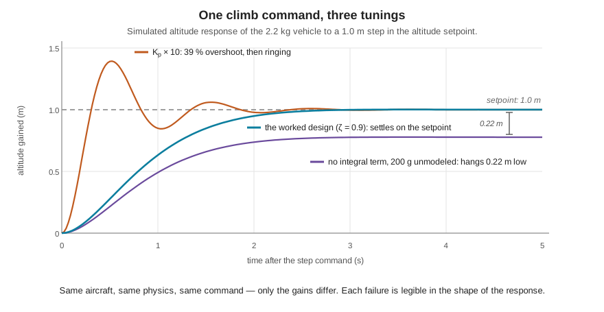
One design, three behaviors, and every one of them legible in the shape of the response — that legibility is why log plots of setpoint against estimate are the primary diagnostic tool for control problems, a thread Part V’s diagnostics material picks up in earnest.
9.6 From Calculus to Code
The law derived above is continuous mathematics; what a flight controller runs is a loop over samples. At each tick \(k\), separated by the sampling period \(\Delta t\), the derivative becomes a difference, the integral becomes a running sum, and the controller becomes a handful of lines executed on the order of a thousand times per second:
def pid_step(setpoint, measurement, dt, state):
    error = setpoint - measurement

    # P: the present error
    p_term = KP * error

    # I: accumulate, but clamp -- see "windup" below
    state.integral = clamp(state.integral + KI * error * dt,
                           -I_LIMIT, +I_LIMIT)

    # D: differentiate the *filtered* measurement, not the raw error
    d_term = -KD * state.deriv_filter.update(measurement, dt)

    return p_term + state.integral + d_term
The differences between this and the textbook equation are not blemishes; they are the accumulated flight experience of every autopilot project, and three of them matter enough to name.
Saturation and integrator windup. Motors have a floor and a ceiling. When the loop commands more than the hardware can deliver — the 3 m step that wants 26 N of the 17.7 N available — the command clips, but a naive integrator keeps accumulating the error the clipped command failed to remove. By the time the vehicle finally reaches the setpoint, the integrator holds a large stale total that must be un-accumulated, and it discharges as a long overshoot on the far side. The fix in the code above is the clamp: bound the integrator so it can never hold more authority than a modest fraction of the actuator range. Production controllers go further (freezing integration while saturated, or back-calculating), but the clamp is the load-bearing idea.
Derivative filtering. Differencing adjacent samples of a noisy signal divides the noise by \(\Delta t\), and at kilohertz rates \(\Delta t\) is small — raw differentiation of a vibrating airframe’s gyro signal produces a derivative term that is mostly amplified vibration, fed straight to the motors as heat and twitch. Every practical implementation low-pass filters the signal before (or while) differentiating it. This is also where the mechanical world reaches into the control law: the propeller balance and frame stiffness the Materials and Power chapter argued for are, among other things, what makes a useful \(K_d\) possible at all.
Derivative on measurement. The code differentiates the measurement rather than the error. When a setpoint changes stepwise — a new altitude command arrives — the error jumps discontinuously, and differentiating it produces a one-sample spike of enormous magnitude (a “derivative kick”) that bangs the actuators for no physical reason. The measurement itself never jumps; differentiating it yields the same damping with no kick. It is a one-line change that every flight stack makes.
9.7 Why One Loop Is Not Enough
Nothing so far explains the architecture the previous chapter promised — so consider trying to fly with a single PID from position error straight to motor commands. The loop must then handle, all at once, dynamics living on wildly different time scales: position responds over seconds, attitude over tenths of a second, angular rate over hundredths. One set of three gains cannot serve all three regimes — tuned tight enough to stabilize the fast rotational dynamics it will be violently aggressive about position errors; tuned gentle enough for position it will be far too slow to catch a tilt. And the coupling runs deeper: because the vehicle is underactuated, a position error does not even correspond to any particular motor command — it corresponds to a desired tilt, which corresponds to a desired rotation, which finally corresponds to a torque.
The architecture that resolves both problems is the cascade, shown in Figure 9.3: a chain of loops, each consuming the setpoint the loop outside it produced and producing the setpoint for the loop inside it, each running faster than the one outside it. This is the structure PX4 implements for multirotors, and its stages map exactly onto the chain of physical implications above.
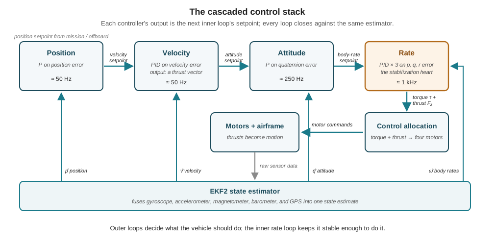
Read the chain left to right as a sequence of translations, each answering one question. The position controller — a plain proportional loop, no I or D — answers where should I be? by converting position error into a velocity setpoint. The velocity controller, a full PID, answers how fast should I move? — and its output is worth pausing on, because it is not a motor command but a thrust vector: a magnitude (how hard to push) and a direction (which way), which is precisely the “translation is bought with tilt” coupling made explicit. The attitude controller answers which way should thrust point? by comparing desired against estimated orientation — as quaternions, not Euler angles, to stay free of singularities — and emitting body-rate setpoints through a proportional law. The rate controller answers how fast should I rotate? and is the innermost loop of the entire vehicle: three independent PIDs, one per body axis, converting rate error into a torque demand at approximately the gyro rate, on the order of a kilohertz. Finally, control allocation solves the geometry problem the Anatomy of a Multirotor chapter set up — given a desired total thrust and three desired torques, choose four motor thrusts, using the motor positions and spin directions, that realize them within limits.
The cascade works because of time-scale separation: each loop runs several times faster than the loop outside it, so from the outer loop’s viewpoint the inner loop is essentially a solved problem — command a body rate, and it simply happens. The discipline this imposes runs both ways. Inner loops must actually be fast and well-tuned, which is why the rate loop is tuned first and best: every flight mode, from full manual to full autonomy, passes through it, and a defect there surfaces everywhere. And outer loops must not ask for motion faster than the inner loops can deliver, which is the control-theoretic root of a rule the previous chapter stated operationally — the mission layer requests, the flight controller disposes.
The cascade is also why the running example’s software never touches a motor. When Part II’s later chapters script the Goose Management System’s search grid, its companion computer will publish position and velocity setpoints into the left end of this chain, and when a detected goose demands the evasive climb whose 7.8 m/s² ceiling the previous chapter computed, that maneuver too will be delivered as setpoints and honored by these same four loops. Where do the gains themselves live? In PX4 they are ordinary named parameters — MC_ROLLRATE_P, MC_PITCHRATE_D, MPC_Z_VEL_P_ACC, and their kin — stored on the flight controller and adjustable without recompiling firmware; the PX4 and the Autopilot Stack chapter maps that parameter system, and the loops above are what its numbers feed.
One trace ties the whole architecture together. A wind gust over the protected area rolls the aircraft: the gyro reports a roll rate that the rate setpoint never asked for; the rate PID sees the error, and its proportional term commands an opposing torque within a millisecond or two while its derivative term brakes the buildup; the allocator converts the torque into four slightly changed motor commands; the airframe rotates back. If the gust is sustained rather than momentary, the attitude loop’s error persists, the position loop watches the vehicle drift downwind, and each outer layer leans its setpoints upwind until the drift stops — the integral terms quietly absorbing whatever steady lean the gust demands. Nothing above the rate loop needed to know the gust happened quickly, and nothing below the position loop needed to know the mission cared. That division of labor, running hundreds of times per second in silence, is what “the flight controller stabilizes the vehicle” actually means.
9.8 Tuning: Reading the Gains from Flight Behavior
Gains are not abstract. Each mistuning has a physical signature, and a practiced eye diagnoses a vehicle from thirty seconds of hover the way a mechanic diagnoses an engine from idle. The table collects the symptoms developed through this chapter.
| Gain | Too low | Too high |
|---|---|---|
| \(K_p\) | Sluggish, soft response; poor tracking; leans with disturbances | Oscillation and twitching; overshoot; high motor activity |
| \(K_i\) | Steady drift; persistent offset never removed | Slow wallowing oscillation; overshoot after saturation (windup) |
| \(K_d\) | Overshoot and ringing; poor damping | Noise amplification; hot motors; vibration sensitivity |
The workflow that turns the table into a safe procedure has a fixed order, and each step exists because of something quantitative from earlier chapters. Mechanics first: balanced propellers, a rigid frame, a sane centre of gravity, correct motor order and spin direction — no gain can compensate for a vibration source feeding the derivative term or a mixer commanding the wrong motor. Then sensors: a calibrated IMU and acceptable vibration metrics, because every loop closes against the estimate. Then start conservative, from published defaults for a similar airframe class. Then tune from the inside out: rate loop first, then attitude, then velocity and position — because every outer loop’s correctness assumes the loops inside it already track well, an assumption the cascade’s whole architecture rests on. Then read the logs, comparing setpoint against estimate for each loop and watching for saturation. Bench tests happen with propellers removed; aggressive tuning happens nowhere near people. The natural place to practice all of this without bending an aircraft is simulation, where the same PX4 code runs against a modeled plant — the subject of this chapter’s related lab.
It is fair to ask why, in an era of model-predictive and learning-based control, a law from the age of steam governs every small multirotor flying. The honest answer is engineering economics: PID is computationally almost free, which matters at a kilohertz on a microcontroller; it is transparent, so a log tells you which term misbehaved; it requires no model of the plant beyond what tuning extracts; and the cascade structure lets a stack of simple loops manage a nonlinear vehicle that no single simple loop could. Its limits are real — performance degrades away from hover, saturation can exceed its authority, and gains tuned for one payload are wrong for another — but within the envelope a multirotor actually flies, it has proven very hard to beat at the price.
The natural next steps beyond PID each relax one of its simplifications. The linear-quadratic regulator (LQR) derives all gains at once from a linearized model by minimizing a stated cost, replacing per-loop hand-tuning with a principled trade between error and effort. Model-predictive control (MPC) re-solves a short constrained optimization every cycle, which lets it respect actuator limits inside the law rather than clamping after the fact — increasingly practical on companion-computer-class hardware for aggressive trajectories. Adaptive and learning-based controllers re-estimate the plant in flight, attacking the payload-changes-the-gains problem directly. Each buys capability with computation and with opacity, which is why the innermost loop of certified and hobby aircraft alike remains, for now, the law of this chapter.
9.9 Check Your Understanding
- The empty research airframe from Part I has a mass of 1.7 kg. Using the same design targets as the worked example (\(\omega_n = 2.0\) rad/s, \(\zeta = 0.9\)), compute the altitude-hold gains \(K_p\) and \(K_d\) — and explain why the gains tuned for the 2.2 kg loaded vehicle are wrong for the empty one.
\(K_p = m\omega_n^2 = 1.7 \times 4 = 6.8\) N/m and \(K_d = 2\zeta\omega_n m = 2(0.9)(2.0)(1.7) = 6.12\) N·s/m. The gains scale with mass because the plant does: the same thrust correction accelerates a lighter vehicle harder. Flying the empty airframe on the loaded vehicle’s gains (\(K_p = 8.8\), \(K_d = 7.92\)) raises \(\omega_n\) to \(\sqrt{8.8/1.7} = 2.28\) rad/s — a stiffer, faster response than designed, though with \(\zeta = 7.92/(2 \times 1.7 \times 2.28) = 1.02\) it stays well damped. The general lesson is the last row of the chapter: gains encode a model of the plant, and changing the payload silently changes the plant.
- A proportional-only altitude controller with \(K_p = 8.8\) N/m faces a steady 3.0 N downdraft. Compute the steady-state error, state which PID term removes it, and name the failure mode that term introduces if the vehicle spends time at full throttle.
At equilibrium the proportional command balances the disturbance: \(K_p e_{ss} = 3.0\) N, so \(e_{ss} = 3.0/8.8 = 0.34\) m below setpoint. The integral term removes it, accumulating command as long as any error persists until the disturbance is fully cancelled at zero error. The introduced risk is integrator windup: if the motors saturate — a long full-throttle climb, or a disturbance larger than the thrust margin — the integrator keeps accumulating error it cannot act on, then discharges as a large overshoot once authority returns. The remedy is to clamp the integrator (or freeze it during saturation).
- A colleague tunes the altitude loop to \(\zeta = 0.5\) to get a faster rise. Compute the resulting overshoot, and explain why that tuning is acceptable for a climb from 30 m to 40 m over open water but unacceptable for a climb commanded to the 122 m regulatory ceiling.
\(M_p = \exp(-\pi\zeta/\sqrt{1-\zeta^2}) = \exp(-\pi(0.5)/\sqrt{0.75}) = \exp(-1.814) \approx 0.163\), so about 16 % overshoot. Overshoot scales with step size: a 10 m climb overshoots by about 1.6 m, harmless with 80 m of sky above. But commanded to the ceiling, the same controller passes 1.6 m per 10 m of step beyond it — the vehicle physically busts the limit before settling back, even though the setpoint itself was legal. Either the damping must be restored toward critical, or the mission layer must leave altitude margin at least equal to the worst-case overshoot — the layered-margin logic of the Airspace Law chapter, now derived from a control parameter.
- Three vehicles misbehave in hover: (a) one twitches rapidly, motors audibly busy, oscillating several times per second; (b) one slowly wanders off altitude and never comes back; (c) one holds attitude but its motors run hot and it reacts violently to the slightest airframe vibration. Diagnose the gain problem in each.
- Excessive \(K_p\) (or insufficient damping relative to it) in a fast loop, classically the rate loop: the fast oscillation is the stiffness/inertia cycle of the chapter’s \(K_p \times 10\) example. Remedy: reduce \(K_p\) or add \(K_d\). (b) Insufficient (or absent) \(K_i\): a steady disturbance — payload offset, weak motor, drift — is being balanced by a permanent error the proportional term cannot remove. (c) Excessive \(K_d\): the derivative term is amplifying high-frequency vibration and gyro noise into motor commands — heat and twitch with no visible attitude error. Remedy: reduce \(K_d\), strengthen derivative filtering, and fix the mechanical vibration source first.
- Explain why PX4 controls a multirotor with a cascade of four loops rather than one PID from position error to motor commands, and why the tuning workflow insists the rate loop be tuned first.
Two reasons. Time scales: position dynamics evolve over seconds while rotational dynamics evolve over hundredths of a second, and no single set of gains can be simultaneously gentle enough for one and fast enough for the other. Underactuation: a position error does not map to any motor command directly — it maps to a desired velocity, which maps to a desired thrust vector (tilt), which maps to desired body rates, which finally map to torque; the cascade makes each translation an explicit loop. Each outer loop treats the inner loop as a solved problem, so the assumption only holds if inner loops genuinely track well — which is why the rate loop, the innermost, is tuned first: every flight mode passes through it, and a rate-loop defect surfaces in all of them.
- The digital controller differentiates the filtered measurement rather than the raw error. Give both reasons, and explain what each failure would look like in flight if the implementation did neither.
Filtering: differencing adjacent samples amplifies high-frequency noise by roughly \(1/\Delta t\), so an unfiltered derivative of a vibrating airframe’s gyro signal is mostly amplified vibration — in flight, hot motors, audible twitching, and sensitivity to propeller imbalance. Measurement instead of error: when the setpoint steps, the error jumps discontinuously, and its derivative is a one-sample spike (“derivative kick”) that slams the actuators at the moment of every new command — in flight, a thump or lurch each time a new altitude or attitude setpoint arrives. The measurement is continuous even when the setpoint is not, so differentiating it gives the same damping with no kick.
9.10 Try It
Part 1 — build the altitude loop and break it. Write a short Python simulation of the worked example: state \((z, \dot z)\), mass 2.2 kg, Euler integration at \(\Delta t = 0.004\) s (250 Hz), thrust command clamped to the real vehicle’s range (\(-21.6\) N to \(+17.7\) N of correction about hover). Implement the digital PID exactly as the chapter’s code sketch has it — clamped integrator, derivative on measurement. First reproduce Figure 9.2’s three curves: the worked design, the \(K_p \times 10\) ringing, and the 200 g steady-state error (add \(-1.96\) N of constant disturbance with \(K_i = 0\), then watch \(K_i = 2\) remove it). Then command a 3 m step with the integrator clamp removed and watch windup happen: the command saturates at 17.7 N, the integrator accumulates through the whole climb, and the vehicle sails past the setpoint. Restore the clamp and measure how much overshoot it saved.
Part 2 — predict, then verify. Before touching a simulator, write down predictions in the symptom language of the tuning table: what should doubling \(K_d\) alone do to the worked design’s response? Halving \(K_p\)? Setting \(\zeta = 0.3\) by computing the required \(K_d\)? Run each in your Part 1 script and check yourself. Prediction-before-experiment is exactly the habit the related lab exercises against a full PX4 software-in-the-loop vehicle, where the same gains live in real firmware parameters.
Related Lab: See Appendix B for the lab assignment that applies this chapter’s concepts.