20 Vector-Based Threat Evasion: The Math of Escape
The previous chapter closed on the mission’s hinge: a detection preempts the search grid, the drone closes on its target, and the deterrence work begins. This chapter is about the moment that plan inverts — when something starts closing on the drone. A territorial goose breaking off from the flock to defend it, another aircraft blundering into the working volume, any object whose track ends where the drone is hovering: the roles of pursuer and pursued swap in a frame or two, and the vehicle that was maneuvering at a target must instantly maneuver away from one. The response has a hard real-time character that nothing earlier in this Part had. A coverage path is computed before takeoff; an A* query tolerates a few milliseconds of thought. An incoming threat at bird speeds allows roughly the time between two heartbeats to notice, decide, and move.
That tempo dictates the mathematics. There is no grid, no graph, no search: the entire computation is a handful of dot products and cross products on six numbers — the threat’s position and velocity relative to the drone’s — cheap enough to re-run at the estimator’s full update rate. And every one of those numbers lives in the local North-East-Down frame the Coordinate Frames chapter established: the threat’s position arrives from the perception stack as a world-frame point (one more of the imperfect world-frame targets that chapter’s pipeline delivers), its velocity is estimated by differencing successive positions, and the escape command leaves as an NED velocity setpoint. Two questions organize the chapter. First, is this thing actually going to hit me? — a prediction problem, answered by a dot product. Second, which way is out? — a geometry problem, and the answer, perpendicular or opposite to the threat’s trajectory, is constructed with a cross product. Both answers are then handed to the state machinery of the next chapter, where they will live inside a state the Finite State Machines and Behavior Trees chapter names EVADE_THREAT — the highest-priority behavior in the mission, entitled to preempt everything else the drone is doing.
20.1 Learning Objectives
- Form the threat vector and the relative velocity from two position–velocity pairs in local NED, and apply the dot-product test \(\mathbf{r} \cdot \mathbf{v}_{rel} < 0\) to decide whether the threat is closing.
- Derive the time of closest approach \(t^*\) by minimizing the squared separation, compute the miss vector and miss distance, and state the three-part trigger — closing, soon, and inside the safety radius — that starts an evasion.
- Explain, via the danger-cylinder picture, why a direction perpendicular to the threat’s trajectory is the geometrically sound escape when the threat is fast, and when a straight retreat (opposite the approach) is the better choice.
- Construct a full 3D evasion vector with two cross products — one perpendicular to both the track and the line of sight, one pointing away from the predicted passing side — including the NED sign check that prevents commanding a dive and the fallback when the geometry degenerates.
- Verify an escape by recomputing the closest approach under the commanded velocity, and state the two assumptions (instant velocity change, non-maneuvering threat) whose failure motivates bounded-acceleration commands and, for a pursuing threat, potential fields or rapid re-planning.
20.2 Key Vocabulary
- Threat vector (\(\mathbf{r}\)) — the position of the threat relative to the drone, \(\mathbf{r} = P_{threat} - P_{drone}\), expressed in local NED; a single vector carrying both the bearing and the range of the danger.
- Relative velocity (\(\mathbf{v}_{rel}\)) — the threat’s velocity minus the drone’s, \(\mathbf{v}_{rel} = \mathbf{v}_t - \mathbf{v}_d\); it collapses two moving trajectories into one straight-line track flown past a drone pinned at the origin.
- Collision course — an encounter that is closing (\(\mathbf{r} \cdot \mathbf{v}_{rel} < 0\)) and whose predicted point of closest approach falls inside the safety radius; either condition alone is not yet an emergency.
- Closest point of approach (CPA) — the moment \(t^* = -(\mathbf{r} \cdot \mathbf{v}_{rel})/\lVert\mathbf{v}_{rel}\rVert^2\) at which the separation between drone and threat is smallest, and the miss vector \(\mathbf{m} = \mathbf{r} + \mathbf{v}_{rel}\,t^*\) describing where the threat passes and by how much.
- Safety radius (\(R_{safe}\)) — the minimum separation the mission is willing to accept between the drone and any uncooperative mover; a predicted miss distance below it is the evasion trigger.
- Evasion vector — the commanded escape direction: perpendicular to the threat’s trajectory when the threat is fast, opposite the approach when the drone can outrun it, and always biased away from the side on which the threat will pass.
- Cross product (\(\mathbf{a} \times \mathbf{b}\)) — the vector perpendicular to both of its operands, with magnitude \(\lVert\mathbf{a}\rVert \lVert\mathbf{b}\rVert \sin\theta\); the constructor of perpendicular escape directions, and identically zero when its operands are parallel — the degenerate case the code must catch.
- Safe altitude — a designated altitude, above the encounter, that the escape maneuver climbs toward; giving the evasion state a fixed destination turns “flee” into a bounded, resumable behavior.
- Potential field — a control technique that sums a repulsive gradient pushed out by each threat with an attractive gradient pulled toward a goal, and commands the net downhill direction; the standard first answer when the threat pursues rather than flying a straight line.
20.3 The Threat Vector and the Closing Test
Everything begins by subtracting. The perception pipeline delivers the threat’s position \(P_t\) in local NED — the same camera-to-world chain of the Coordinate Frames chapter, pointed now at something the mission fears instead of something it seeks — and the flight controller’s estimator supplies the drone’s own position \(P_d\) and velocity \(\mathbf{v}_d\). The threat vector
\[ \mathbf{r} = P_t - P_d \]
compresses the situation into one arrow: its norm \(\lVert\mathbf{r}\rVert\) is the range, its direction is the bearing. But a position, however close, is not yet a threat — a goose ten metres away flying away is scenery. Danger lives in the motion, and the motion that matters is relative. Estimate the threat’s velocity \(\mathbf{v}_t\) (in practice by differencing its last few world-frame positions over their timestamps) and form the relative velocity
\[ \mathbf{v}_{rel} = \mathbf{v}_t - \mathbf{v}_d . \]
This subtraction performs a conceptual simplification worth pausing on: it pins the drone at the origin of a relative frame and lets the threat do all the moving. Two curved, coupled trajectories become one straight line — the threat travels along \(\mathbf{r} + \mathbf{v}_{rel}\,t\) — and every question about the encounter becomes a question about how close that line passes to a fixed point.
The first question is binary: is the gap shrinking? The separation’s rate of change has the sign of the dot product \(\mathbf{r} \cdot \mathbf{v}_{rel}\) — differentiate \(\lVert\mathbf{r}(t)\rVert^2\) and the term \(2\,\mathbf{r}\cdot\mathbf{v}_{rel}\) is what comes out. The test reads directly:
\[ \begin{aligned} \mathbf{r} \cdot \mathbf{v}_{rel} &< 0 \;\Rightarrow\; \text{closing}, \\ \mathbf{r} \cdot \mathbf{v}_{rel} &> 0 \;\Rightarrow\; \text{opening}, \\ \mathbf{r} \cdot \mathbf{v}_{rel} &= 0 \;\Rightarrow\; \text{abeam}. \end{aligned} \]
The intuition is the dot product’s usual one: it measures alignment. A negative value means the relative motion points back along the line of sight — the threat is eating range. Run continuously, this three-way test is the cheapest early-warning system in robotics: three multiplications, two additions, and a sign check per update.
Numbers make it concrete, and the encounter they describe will run through the whole chapter. Mid-mission, the drone holds \(P_d = (30.0,\ 10.0,\ {-10.0})\) — 10 m up, in NED’s negative-down convention — drifting north at \(\mathbf{v}_d = (1, 0, 0)\) m/s. A goose breaks toward it from ahead and to the right: \(P_t = (38.0,\ 12.0,\ {-10.0})\), flying south at \(\mathbf{v}_t = (-3, 0, 0)\) m/s, at the same altitude. Then
\[ \begin{aligned} \mathbf{r} &= (8,\ 2,\ 0), \qquad \lVert\mathbf{r}\rVert = \sqrt{68} \approx 8.25\ \text{m}, \\ \mathbf{v}_{rel} &= (-3-1,\ 0,\ 0) = (-4,\ 0,\ 0)\ \text{m/s}, \\ \mathbf{r} \cdot \mathbf{v}_{rel} &= (8)(-4) + (2)(0) + (0)(0) = -32 \;<\; 0 . \end{aligned} \]
Closing — at \(-(\mathbf{r}\cdot\mathbf{v}_{rel})/\lVert\mathbf{r}\rVert = 32/8.25 \approx 3.9\) m/s, the drone’s 1 m/s of northward drift and the goose’s 3 m/s of southward flight pooled into one number. (The speeds are deliberately leisurely so the arithmetic stays legible; the geometry, not the tempo, is the lesson, and it survives unchanged when the incomer is three times faster.)
20.4 Predicting the Near Miss
Closing is necessary but not sufficient: two aircraft can close for a while and still pass comfortably wide. The evasion decision needs the future minimum of the separation, and for a straight-line relative track that minimum has a closed form. The squared separation at time \(t\) is
\[ d^2(t) = \lVert \mathbf{r} + \mathbf{v}_{rel}\,t \rVert^2 = \lVert\mathbf{r}\rVert^2 + 2\,(\mathbf{r}\cdot\mathbf{v}_{rel})\,t + \lVert\mathbf{v}_{rel}\rVert^2\,t^2, \]
an upward-opening parabola in \(t\). Setting its derivative to zero gives the time of closest approach
\[ t^* = -\,\frac{\mathbf{r}\cdot\mathbf{v}_{rel}}{\lVert\mathbf{v}_{rel}\rVert^2}, \]
which is positive exactly when the encounter is closing — the dot-product test and the CPA formula agree by construction. Substituting \(t^*\) back gives the miss vector, the threat’s position relative to the drone at that worst moment:
\[ \mathbf{m} = \mathbf{r} + \mathbf{v}_{rel}\,t^* . \]
Its norm is the predicted miss distance, and one property of \(\mathbf{m}\) will earn its keep shortly: it is always perpendicular to \(\mathbf{v}_{rel}\) (at the closest point, the relative motion is exactly sideways — that is what “closest” means).
For the running encounter:
\[ \begin{aligned} t^* &= \frac{32}{(-4)^2 + 0 + 0} = \frac{32}{16} = 2.0\ \text{s}, \\ \mathbf{m} &= (8,\ 2,\ 0) + (-4,\ 0,\ 0)(2.0) = (0,\ 2,\ 0), \\ \lVert\mathbf{m}\rVert &= 2.0\ \text{m}. \end{aligned} \]
In two seconds, the goose passes 2.0 m to the drone’s east, at the same altitude. Whether that is an emergency is a mission parameter, not mathematics: the safety radius \(R_{safe}\) encodes how much separation the operator demands from an uncooperative mover — 3 m here, roughly the drone’s rotor span plus a wingspan plus turbulence margin. The full trigger is a three-part conjunction, and each part guards against a different false alarm:
- Closing: \(\mathbf{r}\cdot\mathbf{v}_{rel} < 0\) — otherwise the threat is departing and any maneuver is wasted battery.
- Soon: \(t^* \le T_{horizon}\) (a few seconds) — a threat predicted to arrive in forty seconds will be re-predicted forty times before it matters; acting on distant extrapolations of a noisy velocity estimate produces a drone that flinches at everything.
- Close: \(\lVert\mathbf{m}\rVert < R_{safe}\) — the pass must actually violate the radius.
Here: closing (yes), \(t^* = 2.0\) s (soon), miss \(2.0 < 3\) m (inside). Evade — with two seconds in hand. Figure 20.1 lays the whole prediction out to scale.
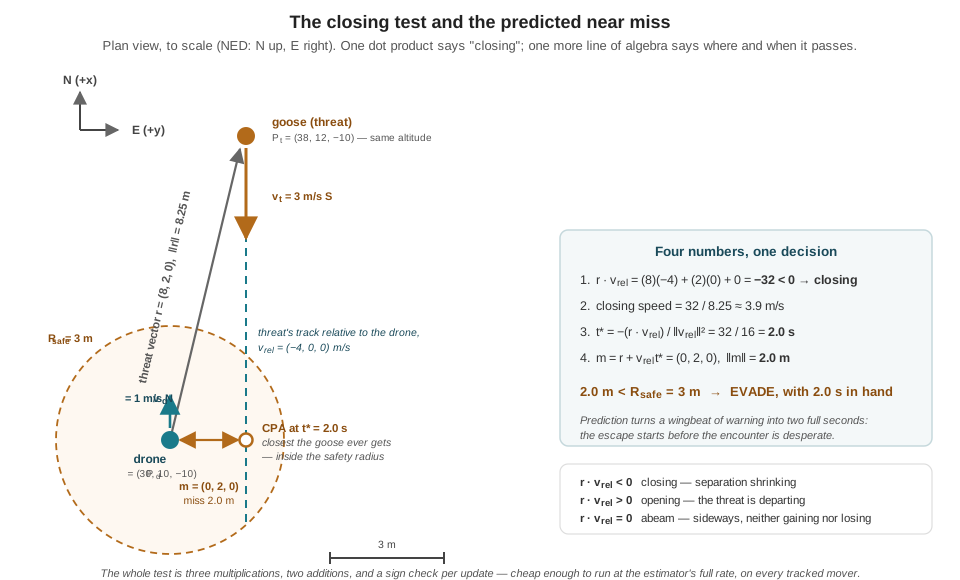
The two-second warning is the entire argument for prediction over reaction, and it deserves the emphasis the numbers give it. A purely reactive system — one that maneuvers when the range gets small — would begin its escape with the goose a wingbeat away, spending its maneuver on desperation. The predictive system starts the same escape 2 s and 8 m earlier, which at quadrotor accelerations is the difference between a brisk sidestep and a stall-the-airframe emergency. The prediction costs almost nothing (the formulas above are a dozen floating-point operations) but it leans on estimates that do cost something: the threat’s position carries the half-metre-scale error the Coordinate Frames chapter budgeted at these ranges, and differencing noisy positions to get \(\mathbf{v}_t\) amplifies that noise. A miss predicted at 2.9 m against a 3 m radius is not meaningfully different from one predicted at 3.1 m — which is why \(R_{safe}\) is chosen with slack in it, and why the assessment re-runs every update rather than trusting any single prediction.
20.5 Why Perpendicular Is the Way Out
The trigger has fired; the drone owns 2.0 seconds. Which way should it go? The lab-honed rule of thumb — escape perpendicular or opposite to the threat’s trajectory — sounds like folklore until it is drawn in the relative frame, where it becomes a theorem about cylinders.
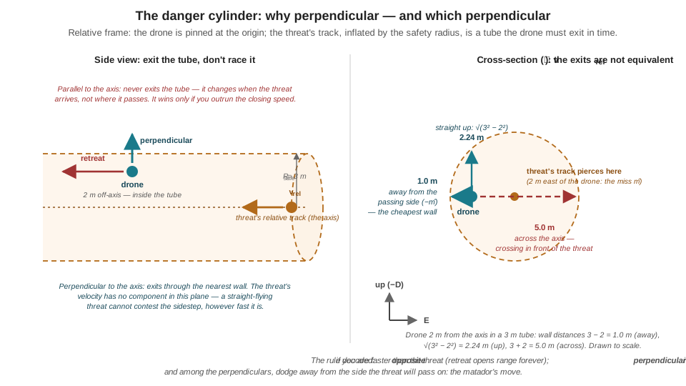
Pin the drone at the origin. The threat travels the straight line \(\mathbf{r} + \mathbf{v}_{rel}\,t\); inflate that line by the safety radius and it becomes a danger cylinder of radius \(R_{safe}\) around the threat’s relative track — the set of every position that will, at some moment, be within \(R_{safe}\) of the threat. The drone is currently inside this cylinder (that is precisely what miss distance \(2.0 < 3\) m means), and escaping is now a literal geometric task: get outside the tube before the threat arrives.
Seen this way, the candidate maneuvers sort themselves:
- Motion parallel to the cylinder’s axis — directly away along the threat’s line of approach — never exits the tube at all. It changes when the threat arrives, not where it passes. If the drone can sustain a higher speed than the threat’s closing rate, this straight retreat opens the range forever and is a perfectly good escape; if it cannot, retreat merely postpones the same near miss. Running from a faster pursuer down its own track is the one provably losing move.
- Motion perpendicular to the axis exits through the nearest wall, and converts every metre-per-second of drone speed into miss distance. Crucially, its effectiveness does not depend on the speed ratio: the threat’s velocity has no component in the perpendicular plane (that is what perpendicular means), so a straight-flying threat cannot contest the sidestep at all. This is the escape that still works when the incomer is faster — and the threats worth engineering for, a territorial goose in full flight or a rogue aircraft, generally are. Rerun the encounter with the goose replaced by a 12 m/s incomer on the same track: \(t^*\) collapses to roughly 0.6 s and the miss distance stays 2.0 m (the miss depends on the track’s direction, not its speed); retreat at any achievable quadrotor speed loses, but the perpendicular exit — 1 m to the nearest wall, as computed next — remains a fraction of a second’s work.
So “perpendicular or opposite” decodes to: opposite if you are faster (it maximizes range and buys time), perpendicular if you are not (it is the only direction the threat cannot defend). A small autonomous drone facing birds and aircraft should assume it is not.
One question remains: perpendicular which way? The perpendicular directions form a whole plane — from inside a tube you can aim at any point of the wall — and they are far from equivalent. The drone sits 2.0 m from the cylinder’s axis (the miss distance is exactly the drone’s distance from the relative track), in a tube of radius 3 m. Exit toward the side the threat will pass on — east, through the axis — and the wall is \(R_{safe} + \lVert\mathbf{m}\rVert = 5.0\) m away, crossing in front of the danger on the way. Exit away from the passing side — west — and the wall is \(R_{safe} - \lVert\mathbf{m}\rVert = 1.0\) m away. Exit straight up, at right angles to the miss, and the chord gives \(\sqrt{R_{safe}^2 - \lVert\mathbf{m}\rVert^2} = \sqrt{9-4} \approx 2.24\) m. The ranking is general: the cheapest exit is directly away from the miss vector — dodge away from the side on which the threat will pass, the matador’s move — with the perpendicular-to-the-miss directions (for a co-altitude encounter, straight up) a respectable second that buys vertical separation and ground clearance. Figure 20.2 makes the picture exact.
20.6 Building the Escape with Cross Products
The geometry says: move in the plane perpendicular to \(\mathbf{v}_{rel}\), biased away from the passing side, and preferably upward. The tool that constructs such directions from the vectors already in hand is the cross product. For \(\mathbf{a} \times \mathbf{b}\), the essentials: the result is perpendicular to both operands; its magnitude is \(\lVert\mathbf{a}\rVert\lVert\mathbf{b}\rVert\sin\theta\); its sign follows the right-hand rule and flips if the operands swap; and it vanishes when the operands are parallel — a failure mode, not a curiosity, that the implementation below must detect. Componentwise,
\[ \mathbf{a} \times \mathbf{b} = \big(a_y b_z - a_z b_y,\;\; a_z b_x - a_x b_z,\;\; a_x b_y - a_y b_x\big). \]
The construction uses it twice, and each application answers one of the geometry’s demands.
First cross product — perpendicular to everything. The two vectors that define the encounter are the relative track \(\mathbf{v}_{rel}\) and the line of sight \(\mathbf{r}\). Their cross product
\[ \mathbf{u}_1 = \mathbf{v}_{rel} \times \mathbf{r} \]
is perpendicular to both: it leaves the collision plane entirely, at right angles to the track (so the threat cannot contest it) and at right angles to the line of sight (so every unit of motion is pure lateral separation). For the running encounter,
\[ \begin{aligned} \mathbf{u}_1 &= (-4,\ 0,\ 0) \times (8,\ 2,\ 0) \\ &= \big( (0)(0)-(0)(2),\;\; (0)(8)-(-4)(0),\;\; (-4)(2)-(0)(8) \big) \\ &= (0,\ 0,\ -8), \qquad \hat{\mathbf{u}}_1 = (0,\ 0,\ -1). \end{aligned} \]
Both defining vectors were horizontal, so their mutual perpendicular is vertical — and in NED, a \(D\)-component of \(-1\) points up. That sign was luck, and luck is not a control law: swap the operand order and the same arithmetic yields \((0, 0, +8)\), a command to dive at the ground. The implementation therefore checks the \(D\)-component and negates the vector if it is positive — both \(\mathbf{u}_1\) and \(-\mathbf{u}_1\) are equally perpendicular, and the mission’s preference between them is not geometric but physical: climb, never dive. Climbing moves away from the ground, the obstacles, and (for an avian threat defending ground it considers its own) usually the contested airspace; it is also the direction of the designated safe altitude the maneuver ultimately makes for.
Second cross product — away from the passing side. \(\hat{\mathbf{u}}_1\) solves the vertical axis of the escape plane; the horizontal axis should point away from the miss. Crossing the track with \(\hat{\mathbf{u}}_1\) produces the remaining perpendicular direction:
\[ \begin{aligned} \mathbf{u}_2 &= \mathbf{v}_{rel} \times \hat{\mathbf{u}}_1 = (-4, 0, 0) \times (0, 0, -1) = (0,\ -4,\ 0), \\ \hat{\mathbf{u}}_2 &= (0,\ -1,\ 0) \end{aligned} \]
— due west, which is exactly \(-\hat{\mathbf{m}}\), the direction away from the goose’s predicted 2 m-east pass. That is not a numerical coincidence. The vector triple product identity \(\mathbf{a}\times(\mathbf{a}\times\mathbf{c}) = \mathbf{a}(\mathbf{a}\cdot\mathbf{c}) - \mathbf{c}\lVert\mathbf{a}\rVert^2\), applied with \(\mathbf{a} = \mathbf{v}_{rel}\) and \(\mathbf{c} = \mathbf{r}\), gives
\[ \begin{aligned} \mathbf{v}_{rel}\times(\mathbf{v}_{rel}\times\mathbf{r}) &= \mathbf{v}_{rel}\,(\mathbf{v}_{rel}\cdot\mathbf{r}) - \mathbf{r}\,\lVert\mathbf{v}_{rel}\rVert^2 \\ &= -\lVert\mathbf{v}_{rel}\rVert^2 \left( \mathbf{r} - \mathbf{v}_{rel}\, \frac{-(\mathbf{r}\cdot\mathbf{v}_{rel})}{\lVert\mathbf{v}_{rel}\rVert^2} \right) = -\lVert\mathbf{v}_{rel}\rVert^2\, \mathbf{m}, \end{aligned} \]
since the parenthesized quantity is precisely \(\mathbf{r} + \mathbf{v}_{rel}\,t^*\). The double cross product is always anti-parallel to the miss vector: the construction does not merely find some perpendicular — it automatically finds the matador’s side, for any encounter geometry, with no case analysis. This is the quiet payoff of doing the escape with vector algebra instead of hand-tuned rules.
One wrinkle rewards a careful look, because it is invisible in this example and a wrong-way dodge in others. The climb-never-dive negation propagates: negating \(\hat{\mathbf{u}}_1\) negates \(\mathbf{v}_{rel} \times \hat{\mathbf{u}}_1\) as well, which would land the sidestep on the wrong side precisely in the encounters where the climb check fired. The implementation therefore pins \(\hat{\mathbf{u}}_2\) against the miss directly — negate it whenever \(\mathbf{u}_2 \cdot \mathbf{m} > 0\) — a check that is a no-op here (the climb check was too) but load-bearing in half of all geometries. Sign conventions compose, and every sign in a control law earns an explicit test.
The evasion vector. Sum the two unit directions and renormalize — an equal blend of “climb” and “away from the pass,” both lying in the plane the threat cannot contest — and scale by the escape speed \(v_{esc}\) the airframe can honestly deliver:
\[ \begin{aligned} \hat{\mathbf{e}} &= \frac{\hat{\mathbf{u}}_1 + \hat{\mathbf{u}}_2}{\lVert \hat{\mathbf{u}}_1 + \hat{\mathbf{u}}_2 \rVert} = \left(0,\ -\tfrac{1}{\sqrt{2}},\ -\tfrac{1}{\sqrt{2}}\right), \\ \mathbf{v}_{cmd} &= 5\,\hat{\mathbf{e}} = (0,\ -3.54,\ -3.54)\ \text{m/s}. \end{aligned} \]
The escape trajectory: from \((30, 10, -10)\), the drone breaks due west while climbing at 45°, perpendicular to the goose’s north–south track, opening toward the safe altitude (15 m, \(D = -15\)) it will hold until the threat clears. Figure 20.3 draws the full construction in three dimensions.
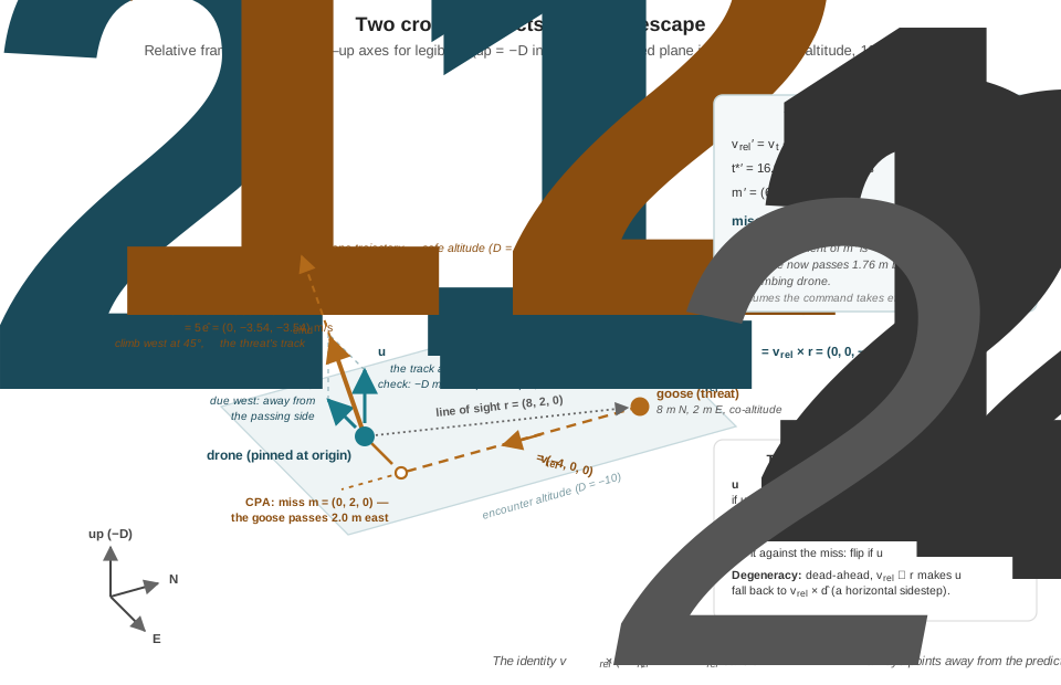
Verify, don’t hope. The construction is only as good as its effect on the number that triggered it, so recompute the closest approach under the commanded velocity. The new relative velocity is \(\mathbf{v}_{rel}' = \mathbf{v}_t - \mathbf{v}_{cmd} = (-3,\ 3.54,\ 3.54)\), and with \(\mathbf{r}\) unchanged at the moment the maneuver begins:
\[ \begin{aligned} \mathbf{r}\cdot\mathbf{v}_{rel}' &= (8)(-3) + (2)(3.54) + 0 = -16.93, \\ t^{*\prime} &= \frac{16.93}{(-3)^2 + (3.54)^2 + (3.54)^2} = \frac{16.93}{34.0} = 0.498\ \text{s}, \\ \mathbf{m}' &= (8, 2, 0) + (-3,\ 3.54,\ 3.54)(0.498) = (6.51,\ 3.76,\ 1.76), \\ \lVert\mathbf{m}'\rVert &= \sqrt{42.3 + 14.1 + 3.1} \approx 7.72\ \text{m}. \end{aligned} \]
The predicted miss climbs from 2.0 m to 7.72 m — from well inside the safety radius to comfortably outside it — and the miss vector’s positive \(D\)-component says the goose now passes 1.76 m below the climbing drone. The encounter still “closes” briefly (the geometry guarantees some approach), but its closest point is a non-event. One honest caveat rides along: this verification assumed the drone’s velocity changed instantly, which no airframe delivers. The next section pays that debt.
The degenerate case. The construction has one hole, and it is the most dangerous geometry of all: a dead-ahead collision. When the threat comes straight down the line of sight, \(\mathbf{r}\) and \(\mathbf{v}_{rel}\) are anti-parallel, \(\mathbf{u}_1 = \mathbf{v}_{rel}\times\mathbf{r} = \mathbf{0}\), and the miss vector is zero too — there is no “side it will pass on” because it will not pass, it will arrive. Geometrically the symmetry is real (every perpendicular is equally good), but code cannot normalize a zero vector, so the implementation substitutes an arbitrary perpendicular: \(\mathbf{v}_{rel} \times \hat{\mathbf{d}}\), with \(\hat{\mathbf{d}} = (0,0,1)\) the NED down axis, gives a horizontal sidestep at right angles to the approach — and if the threat is coming straight down or straight up (making that cross product vanish as well), any horizontal direction serves.
20.7 From Vector to Maneuver
The mathematics compresses into a function small enough to audit line by line — and it must be auditable, because it will run inside the highest-priority behavior in the mission:
import numpy as np

D_HAT = np.array([0.0, 0.0, 1.0])          # NED down axis

def evasion_command(p_d, v_d, p_t, v_t,
                    r_safe=3.0, horizon=5.0, v_esc=5.0):
    """Assess a threat and, if it triggers, return an NED escape
    velocity command; return None if no evasion is required."""
    r = np.asarray(p_t, float) - np.asarray(p_d, float)   # threat vector
    v_rel = np.asarray(v_t, float) - np.asarray(v_d, float)
    closing = r @ v_rel
    if closing >= 0.0:
        return None                        # opening or abeam: no threat
    t_star = -closing / (v_rel @ v_rel)    # time of closest approach
    if t_star > horizon:
        return None                        # closing, but not soon
    miss = r + v_rel * t_star              # CPA miss vector (perp. to v_rel)
    if np.linalg.norm(miss) >= r_safe:
        return None                        # passes outside the radius
    u1 = np.cross(v_rel, r)                # perp. to track and line of sight
    if np.linalg.norm(u1) < 1e-6:          # dead-ahead: no unique side
        u1 = np.cross(v_rel, D_HAT)        # fall back: horizontal sidestep
        if np.linalg.norm(u1) < 1e-6:      # threat vertical: any direction
            u1 = np.array([1.0, 0.0, 0.0])
    if u1[2] > 0.0:                        # NED sign check:
        u1 = -u1                           #   climb, never dive
    u1 /= np.linalg.norm(u1)
    u2 = np.cross(v_rel, u1)               # perp. to the track, in the escape plane
    if u2 @ miss > 0.0:                    # flipping u1 above flips this product too:
        u2 = -u2                           #   re-pin it away from the miss
    n2 = np.linalg.norm(u2)
    e = u1 if n2 < 1e-6 else u1 + u2 / n2
    return v_esc * e / np.linalg.norm(e)   # commanded NED escape velocity
Three implementation realities separate this function from a flying escape.
Bound the command the airframe can honor. The verification above assumed the commanded velocity took effect instantly; a real quadrotor must pitch over and accelerate, and an evasion command that demands an instant 5 m/s reversal — or worse, a naive implementation that converts the evasion vector into an extreme attitude target — will spend its two seconds of warning saturating motors instead of moving. The remedy is the same discipline the cascaded controllers of Part II imposed everywhere else: command velocity, let the position/velocity cascade generate attitudes, and slew the commanded velocity toward \(\mathbf{v}_{cmd}\) under an acceleration cap rather than stepping it. The margin the prediction bought is exactly what pays for the ramp — which is one more argument for triggering on the forecast, not the flinch. One further bound belongs to the mission rather than the airframe: when the threat will pass overhead, the away-from-the-miss direction points downward, and the construction will honestly spend part of the escape descending — correct geometry that the mission’s minimum-altitude margin must be allowed to cap.
Re-run everything, every update. The escape vector is computed from one snapshot of a noisy world. The threat’s velocity estimate wobbles; the threat itself may turn. The evasion state therefore loops the entire assessment at the estimator rate — recompute \(\mathbf{r}\), \(\mathbf{v}_{rel}\), the trigger, and the vector; re-slew toward the fresh command — so that a curving threat faces a continuously re-aimed escape rather than a stale one. Against a straight-flying threat the recomputed vector barely moves and the loop costs nothing; against a maneuvering one, the loop is the difference between a control law and a wish.
Define done. A behavior that can preempt everything needs an exit condition as crisp as its entry: the encounter has cleared when the closing test goes positive and the range exceeds the safety radius with margin — the threat is behind, opening, and far — or when the drone reaches its safe altitude and the threat is no longer tracked. Where control goes next (resume the abandoned search leg? return home?) is sequencing, not geometry, and it is precisely the job of the next chapter: the Finite State Machines and Behavior Trees chapter builds the EVADE_THREAT state around this function — its preemption of every other state on trigger, its guard conditions, and the bookkeeping that lets the interrupted mission resume — turning this chapter’s arithmetic into the reflex arc of the whole system.
Everything above assumes the threat flies straight: the CPA formula extrapolates a line, and the perpendicular escape works because a non-maneuvering threat cannot contest the sideways plane. A pursuing threat breaks both assumptions at once — it re-aims at the drone every instant, so there is no fixed track to be perpendicular to, and any single precomputed escape vector is stale the moment the pursuer turns. The graduate-track extension of this problem replaces the one-shot vector with a continuously recomputed field or plan. The classic tool is the potential field: the threat emits a repulsive potential that grows steeply inside the safety radius, the safe altitude or rally point emits an attractive one, and the drone commands the negative gradient of the sum — recomputed every tick, so the escape direction automatically rotates as the pursuer curves. Potential fields are cheap (a few vector operations per threat, so multiple simultaneous threats just sum) but carry known pathologies: local minima where attraction and repulsion cancel, and oscillation in narrow passages. The heavier alternative is rapid re-planning — re-running a short-horizon planner several times a second over predicted threat positions, in the spirit of the dynamic re-routing discussed with A* in the previous chapter. Between the two sit velocity obstacles, which characterize the set of drone velocities that lead to collision with each mover and choose outside it, and upstream of all of them sits estimation: a pursuer’s future position deserves better than differenced detections, which is where a Kalman filter over the threat’s state earns its place. Against a stochastic pursuer — one that maneuvers unpredictably — the guarantees get weaker and the margins must get correspondingly fatter: the safety radius and trigger horizon absorb what the mathematics no longer promises.
20.8 Check Your Understanding
- A detected mover sits at \(\mathbf{r} = (12, -5, 0)\) m with relative velocity \(\mathbf{v}_{rel} = (2, 1, 0)\) m/s. Apply the closing test and state, in one sentence, what the drone should do about this object.
\(\mathbf{r}\cdot\mathbf{v}_{rel} = (12)(2) + (-5)(1) + 0 = 24 - 5 = +19 > 0\): the separation is growing — the object is departing. The drone should do nothing but keep watching: the test re-runs every update, and a mover that turns will announce itself with a sign change; maneuvering against an opening track wastes battery and interrupts the mission for scenery.
- A threat has \(\mathbf{r} = (10, 0, 0)\) m and \(\mathbf{v}_{rel} = (-3, 1, 0)\) m/s, with \(R_{safe} = 3\) m. Compute \(t^*\), the miss vector, and the miss distance, and make the evade/no-evade call — then say why an engineer might distrust the call either way.
\(\mathbf{r}\cdot\mathbf{v}_{rel} = -30\) (closing); \(\lVert\mathbf{v}_{rel}\rVert^2 = 10\), so \(t^* = 3.0\) s. \(\mathbf{m} = (10,0,0) + (-3,1,0)(3) = (1, 3, 0)\), giving \(\lVert\mathbf{m}\rVert = \sqrt{10} \approx 3.16\) m. Strictly \(3.16 \ge 3\): no evade. But the margin is 16 cm against a position estimate carrying half-metre-scale error and a velocity estimate built by differencing it — well inside the noise. This is exactly why the safety radius is chosen with slack, why the prediction re-runs continuously rather than being trusted once, and why a mission designer might add hysteresis (trigger at 3 m, stand down at 4 m) so the decision doesn’t chatter across the boundary.
- For the encounter of question 2, compute \(\mathbf{u}_1 = \mathbf{v}_{rel}\times\mathbf{r}\) and \(\mathbf{u}_2 = \mathbf{v}_{rel}\times\hat{\mathbf{u}}_1\) (after the NED sign check), and confirm that \(\mathbf{u}_2\) points away from the miss vector you found.
\(\mathbf{u}_1 = (-3,1,0)\times(10,0,0) = \big((1)(0)-(0)(0),\ (0)(10)-(-3)(0),\ (-3)(0)-(1)(10)\big) = (0,0,-10)\). The \(D\)-component is already negative (up), so the sign check passes: \(\hat{\mathbf{u}}_1 = (0,0,-1)\). Then \(\mathbf{u}_2 = (-3,1,0)\times(0,0,-1) = \big((1)(-1)-0,\ 0-(-3)(-1),\ 0\big) = (-1,-3,0)\) — exactly \(-\mathbf{m}\) for the miss \(\mathbf{m} = (1,3,0)\) of question 2, as the triple-product identity guarantees: the construction dodges away from the side the threat passes on, with no case analysis.
- A threat approaches with \(\mathbf{r} = (5, 5, 0)\) and \(\mathbf{v}_{rel} = (-2, -2, 0)\). Compute the miss vector and \(\mathbf{v}_{rel}\times\mathbf{r}\), explain what has happened geometrically, and state what the implementation does about it.
\(t^* = 20/8 = 2.5\) s and \(\mathbf{m} = (5,5,0) + (-2,-2,0)(2.5) = (0,0,0)\): a predicted dead-center collision. The cross product also vanishes — \(\mathbf{v}_{rel}\times\mathbf{r} = (0, 0, (-2)(5)-(-2)(5)) = \mathbf{0}\) — because \(\mathbf{r}\) and \(\mathbf{v}_{rel}\) are anti-parallel: the threat is coming straight down the line of sight, so there is no “side it will pass on” and every perpendicular is equally good. Code cannot normalize a zero vector, so the implementation falls back to \(\mathbf{v}_{rel}\times\hat{\mathbf{d}}\) (a horizontal sidestep perpendicular to the approach), and if the threat’s track is itself vertical, to any fixed horizontal direction. The most symmetric geometry is the most dangerous one, and it is handled by explicit fallback, not by hoping the norm is never small.
- The chapter’s escape blended “climb” and “away from the pass” equally, yielding a 7.72 m verified miss — yet a pure westward sidestep at the same 5 m/s yields about 7.9 m, slightly better. Why might the mission still prefer the blend?
Because miss distance against this threat is not the only currency. The climb component buys vertical separation (the goose passes below, not beside), moves the drone away from the ground and low obstacles just as an aggressive lateral maneuver makes position error most likely, and makes progress toward the designated safe altitude that defines the maneuver’s endpoint — turning “flee” into a bounded behavior with a destination. The pure sidestep optimizes a single scalar; the blend spends a fraction of a metre of miss distance on robustness. Both live in the plane perpendicular to the threat’s track, which is the property that actually defeats the threat.
- Explain why the evasion vector is recomputed at the estimator’s full rate rather than executed once, giving one reason rooted in estimation and one rooted in the threat’s behavior — and name the class of threat for which even a recomputed vector is not enough.
Estimation: the threat’s velocity comes from differencing noisy world-frame positions, so any single snapshot can be badly wrong; re-running the assessment averages the decision over many estimates instead of betting the airframe on one. Behavior: the CPA extrapolation assumes a straight track, so if the threat turns, the old escape vector points the wrong way; the recomputation loop continuously re-aims the escape at the current geometry. The class that defeats both: a pursuing threat, which re-aims at the drone every instant — there is then no fixed track to be perpendicular to, and the tools become potential fields, velocity obstacles, or rapid re-planning, with a filter (e.g., Kalman) improving the threat-state estimate underneath all of them.
20.9 Try It
Part 1 — implement, reproduce, then attack it with randomness. Implement evasion_command() exactly as specified, plus a helper cpa(r, v_rel) returning \((t^*, \mathbf{m})\). Reproduce the chapter’s encounter — drone \((30,10,-10)\) at \((1,0,0)\) m/s, threat \((38,12,-10)\) at \((-3,0,0)\) m/s — and confirm every intermediate: \(\mathbf{r}\cdot\mathbf{v}_{rel} = -32\), \(t^* = 2.0\) s, miss 2.0 m, \(\mathbf{u}_1 = (0,0,-8)\), \(\mathbf{v}_{cmd} = (0,-3.54,-3.54)\), and a verified post-maneuver miss of 7.72 m. Then Monte Carlo it: generate ten thousand random encounters (positions in a 40 m cube, speeds up to 15 m/s), and assert three invariants on every triggering case — the returned command is perpendicular to \(\mathbf{v}_{rel}\) to numerical precision; its sidestep opposes the predicted pass, \(\mathbf{v}_{cmd} \cdot \mathbf{m} \le 0\); and, for encounters that begin from hover, the recomputed miss under the command is never smaller than the unassisted miss. Then relax the hover restriction and study the violations that appear rather than suppressing them: a drone already moving fast in a favorable direction can lose ground when the command discards that velocity for a fixed-speed escape (a case for scaling \(v_{esc}\), not for trusting momentum), and a threat passing far overhead draws a descending dodge that a mission altitude floor must cap. Log the near-degenerate geometries (smallest \(\lVert\mathbf{u}_1\rVert\) before fallback) and check the fallback fired. A control law that survives ten thousand random geometries — including the ones that expose its assumptions — is trustworthy in a way a worked example alone is not.
Part 2 — close the loop in simulation. Move the function into a simulated encounter: propagate a straight-flying threat and a drone that, on trigger, slews its velocity toward the command under a 3 m/s² acceleration cap (the bound a real airframe imposes), re-running the full assessment at 20 Hz. Plot both 3D trajectories and the separation-versus-time curve, marking the trigger instant, the unassisted CPA prediction, and the actual minimum separation achieved — then sweep the trigger horizon from 0.5 s to 5 s and plot achieved miss distance against warning time, which makes the price of late detection quantitative. Finally, make the threat pursue: re-aim its velocity at the drone’s current position each tick and watch the fixed-vector escape degrade as pursuit speed rises. Three sentences: at what pursuer speed does the perpendicular escape stop clearing the safety radius, and which For More technique would you reach for first, and why? In SITL, the same loop runs against PX4 with the command streamed as an Offboard velocity setpoint — the configuration the related lab’s threat-injection exercise grades.
Related Lab: See Appendix B for the lab assignment that applies this chapter’s concepts.